Munich Personal RePEc Archive
How Representative are Representative
Workers? An Assessment of the
Hypothetical Workers Commonly Used
in Social Security Studies
Pfau, Wade Donald
June 2009
Online at
https://mpra.ub.uni-muenchen.de/19036/
This paper was published as:
Pfau, W. D., “How Representative are Representative Workers? An Assessment of the Hypothetical Workers Commonly Used in Social Security Studies,”Journal of Income Distribution. Vol. 18, No. 2 (June 2009), p. 92-117.
It also exists as a working paper:
Pfau, W. D., “The Applicability of Hypothetical Workers for Defined-Contribution Pensions,” GRIPS Discussion Paper 07-11. Tokyo: GRIPS.
“Assessing the Applicability of Hypothetical Workers for Defined-Contribution Pensions”
Wade D. PFAU
Associate Professor
National Graduate Institute for Policy Studies
7-22-1 Roppongi, Minato-ku
Tokyo, JAPAN 106-8677
E-mail: [email protected]
ABSTRACT
An understanding of the financial and distributional consequences of Social Security reform requires knowledge about the actual life circumstances of participants, including the level and pattern of their lifetime earnings and when they retire. Some analyses of Social Security reform make simplifying assumptions about these characteristics by using “hypothetical workers” with set career paths. We seek to develop greater understanding about actual lifetime earnings patterns to compare with hypothetical workers and find discrepancies which lead typical hypothetical workers to produce a more favorable impression for defined-contribution pension reforms. We suggest modifications to make a more suitable hypothetical worker.
Key words: Social Security, Hypothetical Workers, Defined-Contribution Pensions
INTRODUCTION
An understanding of the financial and distributional consequences of Social Security reform requires knowledge about the actual life circumstances of those participating in the Social Security system. This is especially the case with defined-contribution pensions, in which both the level and pattern of lifetime earnings, including when work begins, how many working-age years are spent outside of the labor force, and when work ends, will play instrumental roles in determining benefit amounts. In particular, with a defined-contribution pension, earnings that come early in one’s career will have more time to experience compounding growth. At the same time, the pattern and timing of earnings does not play much role in the formulas used by the United States Social Security Administration (SSA) to calculate the Average Indexed Monthly Earnings (AIME) and the Primary Insurance Amount (PIA), which provide the basis for calculating a worker’s Social Security benefit.
Because obtaining the lifetime earnings data of actual workers for research purposes has been challenging until recently, past researchers often relied on “hypothetical workers” with simplified characteristics for use in studying reform. Hypothetical workers are generally noted for having steady earnings across lengthy careers of forty years or more. They tend to vary only on the basis of earnings levels, gender, marital status, and birth cohort. Gender differences are noted mainly for different mortality rates, not for different earnings levels.
While hypothetical workers can be suitable for studying some aspects of Social Security, such as calculations of “money’s worth” measures, they may fare less well in other regards. We identify defined-contribution pensions as an area in which hypothetical workers may
dramatically overestimate the potential portfolio accumulations, and this paper seeks to examine the issue more closely. While other sources of data are increasingly becoming available for the United States so that using hypothetical workers is no longer necessary, this study still provides an important message for countries that must rely on hypothetical workers for lack of adequate alternatives, such as the recent 53 country study by the World Bank in Whitehouse (2007). Our research suggests how hypothetical workers can be modified to provide better results.
Consequently, reforms which create defined-contribution individual accounts will tend to show larger portfolio accumulations for hypothetical workers than are possible for actual
workers. For example, compared to a hypothetical worker with a lifetime income adjusted to match each actual worker, but with a steady pattern of earnings from age 21 through retirement at 65, the median actual worker from the lowest income decile could only accumulate 65.5 percent as much, and there are very few cases in which actual workers can do as well as the hypothetical worker. Our findings do suggest some hope for hypothetical worker studies though: if hypothetical workers are adjusted to have a scaled-earnings pattern that better matches the actual age-wage profile, and if hypothetical workers are assumed to retire at the early retirement age of 62, then their asset accumulations will much more closely match those of actual workers. Essentially, hypothetical workers have careers spanning too many years and have too much earnings in the early parts of their careers. The goal of this paper is to quantify some of these features in comparing the work histories of actual workers to their hypothetical worker counterparts.
BACKGROUND
Using hypothetical workers to analyze “money’s worth” and redistribution issues in Social Security has a lengthy tradition. In considering some of the more recent incarnations for the United States, Nichols, Clingman, and Glanz (2001) use hypothetical worker models to assess whether different types of workers are able to obtain their “money’s worth” from their contributions to Social Security in terms of rates of return or net lifetime transfers. Their methodology is updated in Clingman and Nichols (2007). Steuerle and Bakija (1994) use hypothetical workers to examine the redistribution of income caused by Social Security both within and across generations. Goss and Wade (2002) use scaled-earnings hypothetical workers who start work at age 21 and retire at age 65 to assess the impact on total portfolio accumulations and benefits of reform proposals that would create defined-contribution individual accounts. Pfau (2003) considers the impact of various Social Security reform proposals based on how they affect hypothetical workers in a stochastic setting. Additionally, while studies about the United States have been shifting toward the use of alternative sources of data on lifetime earnings, the hypothetical worker approach is still used for other countries where alternative data sources are less available. For example, Whitehouse (2007) uses hypothetical workers to compare the defined-benefit and defined-contribution pension systems of 53 countries. These are some of the more recent studies, though Leimer (1999) provides more details about previous incarnations, and Leimer (1995) includes a lengthy bibliography of previous hypothetical worker studies.
Typically, hypothetical workers vary by birth year, gender, level of annual earnings, marital status, and number of children. The breakdown may include four different family types for each of four income levels. Though there is some variation among these details, the family types often include single males, single females, married couples in which the male is the only wage earner, and married couples in which each spouse earns wages. Married couples may be assumed to be the same age as one another and to have children at ages 25 and 30. Thus far, the assumptions are relatively innocuous. Though they are unlikely to describe the exact situation of any particular worker, these assumptions provide a realistic framework for comparison.
traditional pattern is to assign a worker to an earnings level that is some fixed percentage of the economy-wide average earnings level, known as the Average Wage Index (AWI), and then assume that workers earn the same steady proportion of the AWI for their entire career. Because the AWI has historically grown faster than consumer prices, this pattern assumes real wage
growth over one’s career in the neighborhood of one percent per year. Earnings are either low, average, high, or at the maximum taxable level allowed under the Social Security payroll tax. Low wage workers earn 45% of the AWI for each year they work (consistently low wages across a long career), while average wage workers earn the AWI, high wage workers earn 160% of the AWI (up to the maximum taxable wage, which was lower than this in the 1950s and 1960s), and maximum wage workers earn the maximum taxable wage for each year. No distinctions are made by gender with regard to wages. Hypothetical workers typically begin work on their 21st or 22nd birthday and retire on their 62nd (early retirement age) or 65th (full retirement age for those born before 1938) birthday. It is not common to build in periods of unemployment (except for some studies that incorporate disability) for hypothetical workers, and so a constant work history is assumed. One ameliorative feature of the Nichols et al. (2001) study was its creation of a scaled-earnings history to be compared to the traditional steady-earnings history, in which wages follow the well-demonstrated age pattern of starting low at the beginning of one’s career,
rising steadily into one’s 50s, and then slowly descending until retirement. But this approach also does not allow for periods of unemployment.
Practitioners of hypothetical worker studies are well aware of their limitations, which are outlined well in Leimer (1995). He argues that actual workers differ by ages of labor force entry, labor force participation and unemployment patterns, lifetime earnings patterns, ages of
retirement, and survival probabilities, all of which affect the answers to research questions but do not get properly considered in hypothetical worker analyses. These matters may be quite
important when considering potential Social Security reforms. Hypothetical worker studies may introduce biases when the impact of reform depends on the level and pattern of lifetime earnings, as is particularly the case with a defined-contribution pension system. Nonetheless, because of difficulties in obtaining data on the lifetime earnings of workers, researchers have traditionally appealed to the hypothetical worker approach for the lack of better alternatives.
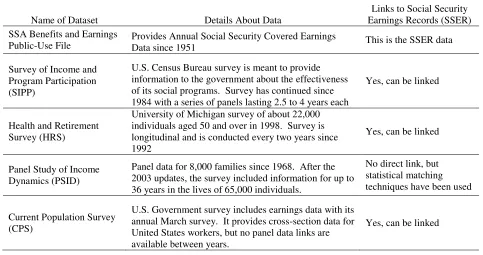
That being said, the past ten years have been witness to an emerging literature which takes care to account for the heterogeneity found in realistic lifetime earnings histories for the United States. Table 1 provides an overview of some of the datasets used for these analyses. The first entry in the table is the SSA Benefits and Earnings Public-Use File, which is more commonly known as the Social Security Earnings Records (SSER). Various versions of this data provide an annual earnings breakdown for Social Security participants since 1951. The data is for Social Security covered earnings, which consists of earnings up to the taxable maximum for workers in jobs covered by Social Security. By linking another dataset to the SSER, researchers have been able to obtain long portions of career earnings for many individuals, for whom they can identify various socioeconomic characteristics. Many studies, though, require researchers to
make artificial extrapolations for missing years of earnings and/or for the worker’s retirement
// Table 1 About Here //
Table 1 also describes some of the key microdatasets which have been linked with the SSER data. These data links are made using Social Security Numbers and are highly restricted for the purposes of confidentiality. An early dataset of this nature is the 1973 Current Population Survey CPS-IRS-SSA Exact Match study, repeated again in 1978. But by 1978, there were only 27 possible years of earnings (1951 to 1977), not yet enough for a full career. More recent incarnations of this approach have matched the Survey of Income and Program Participation (SIPP) or the Health and Retirement Survey (HRS) to the SSER. For example, by linking the 1990-1993 SIPP surveys with Social Security data, Bosworth, Burtless, and Steuerle (1999) investigate the lifetime pattern of earnings, dividing workers into nine groups based on the level (low, average, or high) and shape (rising, level, or declining over time) of lifetime earnings. They find that the pattern assumed by hypothetical workers studies is not typical, and that only 3.4 percent of men and 5.4 percent of women can be classified as middle income workers with level lifetime earnings. Likewise, Au, Mitchell, and Phillips (2004) use the HRS matched to SSA earnings data to assess how well hypothetical workers reflect the earnings histories of actual workers. They find that the earnings of hypothetical workers are larger than actual workers, and that actual workers had more in common with low wage hypothetical workers than with average wage hypothetical workers. In another study, Haider and Solon (2006) use the 1951-1991 Social Security earnings histories linked to the HRS to demonstrate the dangers of using current
earnings to proxy for lifetime earnings and to develop a deeper relationship between annual and lifetime earnings.
Another popular option has been to use the Panel Study of Income Dynamics (PSID), which provides an ongoing panel of 8,000 families since 1968. It can now provide an earnings
record for a large part of a worker’s career. Though it does not cover as long a timeframe, its advantages include its coverage of all earnings (not just Social Security covered earnings) and its linking of spouses. For instance, Coronado, Fullerton, and Glass (1999) use the PSID to
extrapolate lifetime earnings for a sample of individuals with 22 years of earnings observations (1968-1989) in order to more carefully examine Social Security’s redistributive impacts across the lifetime income distribution. Also, Hungerford (2003) took steps to better understand the situation of workers with low lifetime earnings: do they tend to have high annual earnings during a short career, or consistent low annual earnings across a long career? He combines the 1978 Exact Match study with the PSID using statistical matching techniques in order to obtain artificial entire career records. He finds that most workers with low lifetime earnings are women, and the reason for the low lifetime earnings is because of fewer years worked.
Cohen, Steuerle, and Carasso (2001) use the MINT study to analyze the “money’s worth” from
Social Security groups with different socioeconomic characteristics, extrapolating for late-career earnings and retirement ages for younger cohorts. Similarly, Smith, Toder, and Iams (2001) study redistribution issues for Social Security, and with the MINT data they are able to account for spousal earnings as well when studying impacts on the income distribution.
A final approach is microsimulation modeling, in which an artificial collection of individuals is simulated using the relationships estimated from a microdataset. For instance, Harris, Sabelhaus, and Schwabish (2006) explain a way to project labor force participation and earnings for future workers in order to test the implications of different Social Security reforms. In a separate study, Caldwell et al. (1999) use a microsimulation model with an artificial
population generated from the 1960 U.S. Census Public-Use Microdata Sample to study redistribution issues.
DATA AND METHODOLOGY
The data for this study is the Social Security Administration’s Benefits and Earnings
Public-Use Files from 2004. The data includes a random sample of one percent of all recipients of Old-Age, Survivors, and Disability Insurance (OASDI) benefits in December 2004. This amounts to having earnings histories for 406,993 people. Data about the benefits includes the type of benefit, the Primary Insurance Amount (PIA) that serves as the basis for determining
one’s benefit, and the monthly benefit received, as well as other details about whether the recipient was eligible for more than one type of benefit. Data about the beneficiaries includes their year of birth, sex, year of current entitlement, and also the Social Security covered earnings (up to the taxable maximum) of the worker who qualified for the benefit aggregated between 1937 and 1950, and then for each year between 1951 and 2003. For example, if an observation consists of a child qualified for a survivor’s benefit from a deceased parent, then the parent’s earnings record is included in the observation. The data provide a large sample of entire lifetime earnings records for men and women without needing to rely on simulated earnings forecasts for missing years.
The Social Security Administration’s Benefits and Earnings Public-Use Files from 2004 are used to extract the lifetime earnings histories of 113,513 beneficiaries who were born between 1933 and 1942, who did not have earnings before 1951, and who qualified for
retirement benefits at least in part on their own earnings records. This eliminates those receiving disability benefits or other benefits only as a dependent. But it includes spouses who obtain a
benefit partially from their own earnings record as well as their spouse’s earnings record. Also, because disability benefits automatically transition into retirement benefits at the full retirement age, the sample includes some such people who qualified for retirement benefits through
disability.
To consider a worker’s position in the income distribution, we will use a measure of
that boost the wages for later cohorts. For results shown in this paper, we use a discount rate of 3 percent, though we have also checked our results for other discount rates and do not find major qualitative differences in the outcomes. The discount rate can be thought of in real terms, since our wage normalization removes the impacts of general wage growth in the economy.
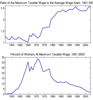
The main advantage of this data is that it provides lifetime earnings for the entire careers of already-retired workers without the need to estimate missing earnings for any part of the workers’ careers. But there remain several limitations for the effectiveness of this data. First, Social Security covered earnings are all that is included, which means that some people may show zero earnings in years when they switched to employment not covered by Social Security. The extent of this problem is hard to quantify, but it is unlikely that people switch frequently between covered and uncovered employment, and Fullerton and Mast (2005) include evidence that over 90 percent of the labor force has been covered by Social Security since the 1970s. However, earnings in the dataset are unfortunately topcoded at the maximum taxable level. This is particularly troublesome in the 1950s and 1960s, when the lack of adjustments for inflation led the maximum taxable wage to be less than 40 percent larger than the average wage, as can be seen in Figure 1. The closest point between maximum taxable and average earnings occurred in 1965, when the AWI was $4659 and the maximum taxable earnings were $4800. Since 1980, the maximum taxable earnings have been at least double the value of the AWI, and they stand at $90,000 in 2005.
// Figure 1 About Here //
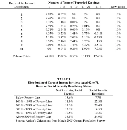
Figure 1 also shows the percent of workers in the sample who earned the maximum taxable earnings for each year between 1951 and 2003. In the 1960s, 25 to 30 percent of workers had incomes at least as large as the maximum table earnings, but the percentage has gradually fallen since then and is presently only a few percentage points. This is an unfortunate situation for our analysis, but the biases created by this data limitation should be somewhat limited. First, the censored earnings will likely not have much impact on the ordering of individuals in the lifetime income distribution. This is because as we move up the income distribution, we find more cases of censored earnings, which will proxy for more earnings in the general ordering of individuals. Next, the censored earnings will bias our analysis of individual accounts because earnings are more censored in the early part of careers, which leads to an appearance of an upward trend in lifetime earnings that is more pronounced than reality for those affected by income censoring. To the extent that this occurs, it will reduce the portfolio value accumulated in the defined-contribution individual account because there will be less earnings in the early part of one’s career to benefit from compound interest. Nevertheless, this problem will be limited for workers in the lower part of the income distribution who rarely tend to earn the taxable
maximum, and it will mostly only affect workers in the top part of the income distribution. Table 2 provides more information about this situation by dividing the income distribution into ten deciles, and showing the breakdown of individuals based on the number of years of topcoded earnings for each decile of the distribution. Half of the sample does not have any censored earning during their careers. We do not otherwise attempt to impute missing earnings, for reasons related to the data limitation that will be described next.
Another limitation of the data is a lack of any socioeconomic characteristics beyond the year of birth and gender. For instance, there is no data on education or race. Obtaining this information would require a link between our data and a previously described survey such as the SIPP, HRS, or CPS. This lack of information leaves out potential explanatory variables in any attempt to impute earnings beyond the maximum taxable level, and it prevents the classification of beneficiaries by such characteristics. Otherwise, it does not create an impediment to studying the characteristics of the lifetime earnings of actual workers and how these characteristics may potentially affect the returns from defined-contribution individual accounts. More importantly, though, marital status is not included in the data. Marital status can be inferred for those people who receive spousal benefits, though such people could be divorced, but the marital status is completely unknown for anyone who is not earning some form of a spousal benefit. This prevents an examination of lifetime earnings within a household. It also means that some
individuals we classify as low-income may actually be living in wealthy households as a result of high spousal earnings or other income-generating assets. We must stress that this applies
throughout the paper, as our analysis of the lower part of the income distribution may include some such individuals.
Another limitation of the data is related to cohort effects, as the lifetime earnings
situation of those in our sample (born between 1933 and 1942) may not produce results that can be generalized to more recent cohorts. In particular, Toder et al. (2002) finds in the MINT study that in recent years women have experienced increasing labor force participation, and in
particular young women in their 20s no longer experience a dip in their employment rates. This will tend to make current earnings differences between men and women less pronounced than in the past. But with this study, we seek to examine lifetime earnings patterns without using assumptions to extrapolate the earnings of a partial career, and lifetime earnings for the younger cohorts are not yet available.
Furthermore, it must be clear that this dataset does not contain a random sample of the U.S. population. The sample contains data only for those who actually receive Social Security benefits in December 2004. For people of retirement age, the sample is biased to look richer because it excludes people who have already died before December 2004, as researchers have demonstrated an inverse relationship between income and mortality since Kitagawa and Hauser (1973), and people who did not earn enough to qualify for Social Security benefits on their own earnings records. But the sample is biased to look poorer because it does not include those people who are still working and who have not begun to collect benefits.
range were not born in the United States. For such individuals, only 53.4 percent were receiving Social Security benefits, compared to 72.2 percent of native born residents. Finally, we find evidence that those not receiving Social Security benefits include a combination of relatively low-income and high-income individuals. Table 3 shows that the family incomes of those not receiving benefits fall more heavily below the poverty line, as well as at least five times above the poverty line, than do the family incomes of Social Security recipients.
// Table 3 About Here //
Also relevant is that it would be a mistake to assume that the historical wage distribution in 1963, for example, would be the same as the wage distribution shown in the data. The data sample of earnings from 1963 may be quite different, since being in the sample requires that you be a recipient of Social Security benefits in December 2004.
RESULTS
The data will be analyzed according to various characteristics related to lifetime earnings patterns to assess the comparability between actual workers and their hypothetical counterparts. These characteristics include retirement ages, the number of years worked, and earnings patterns by age. An important policy implication of the data will also be considered with respect to reforms that would create defined-contribution personal retirement accounts. Distinctions will be made on the basis of age, gender, and position in the income distribution.
Age of Initial Social Security Retirement Benefits Receipt
Hypothetical worker studies generally assume that workers retire at their full retirement age (FRA) or at age 62. For workers born before 1938, the FRA is 65. It is now in the process of increasing, and for those born since 1960, it is 67. With the sample including those born between 1933 and 1942, the FRA ranges from 65 to 65 and 10 months. Workers can collect retirement benefits using their own earnings record starting at age 62, though these benefits are reduced to account for the amount of time before the FRA. Additionally, delays up to age 70 can lead to an increase in annual benefits to compensate for the benefits sacrificed by the delay. There is no financial incentive to delay benefit receipt beyond age 70 though. While the retirement age assumption does not matter to the extent that these benefit reductions and additions are calculated to be actuarially fair, it does matter because delaying one’s retirement probably occurs as a result of continuing employment, which can raise lifetime income and provide more time for growth in a defined-contribution account. As such, it is instructive to examine some characteristics of the age in which workers begin to collect Social Security retirement benefits.
percent began at age 63, 5 percent at age 64, and 28 percent at age 65, which reflects the FRA for everyone in the sample. Only 3 percent of these workers delayed their retirements beyond age 65. One must keep in mind with this result, though, that people who were not yet collecting their benefits in December 2004 are not included in the sample, so that the age distribution just
described is biased in the downward direction. To give some idea about this, the Committee on Ways and Means (2004) provides the distribution of new beneficiary ages for different calendar years and finds, for instance, that 4 percent of new beneficiaries in 1985 were aged 66 and older, and this amount rose to 17.8 percent in 2001.
// Figure 2 About Here //
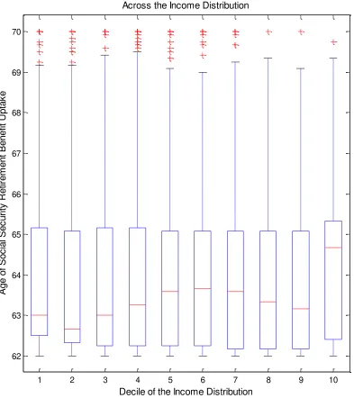
Figure 2 examines the relationship between one’s position in the lifetime income
distribution and the age in which retirement benefits begin. Note that the boxes in Figure 2 and others show the median and interquartile range, and the whiskers are extended to the distance of 1.5 times the length of the interquartile range. The “+” signs beyond the whiskers represent any remaining outliers. The figure displays a weak trend that wealthier individuals retire at later ages, though the median retirement age for each income decile is below age 64, except for the top decile. If lower earners tend to retire at younger ages, then the implication for potential personal retirement accounts would be underperformance because of fewer years for assets to accumulate interest.
Number of Years Worked
Hypothetical worker studies typically assume that workers have careers spanning at least 40 years. Workers are assumed to begin their careers at age 21 or 22 and continue until either age 62 (the earliest age to receive reduced retirement benefits) or age 65 (the historical full retirement age). Meanwhile, the Social Security benefit computation formula uses the top 35 years of earnings in covered employment since age 21 to calculate the worker’s AIME. Working less than 35 years will result in lower benefits than would be implied by such hypothetical
worker studies. Fewer years of work would also mean less contributions to any individual account than would be assumed by the hypothetical worker study.
// Figure 3 About Here //
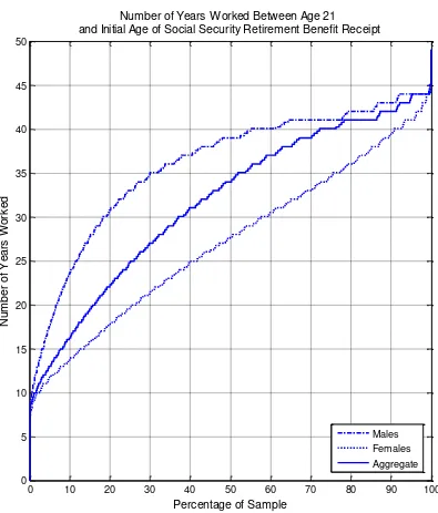
Figure 3 shows the distribution of years worked between age 21 and the age that
retirement benefits began for all of the workers in the sample, also separated by gender. While workers must contribute for at least 10 years to receive retirement benefits, some workers become disabled after fewer years of work and can roll their disability benefits over into retirement benefits at their FRA. Thus, the distribution ranges from less than 10 years of work up to more than 45 years of work. Importantly, for the combined genders, less than 50 percent of retirees have worked at least 35 years, about 40 percent have worked for less than 30 years, and about 25 percent have worked for less than 25 years. Separated by gender, about 30 percent of men work less than 35 years, but almost 75 percent of women work less than 35 years.
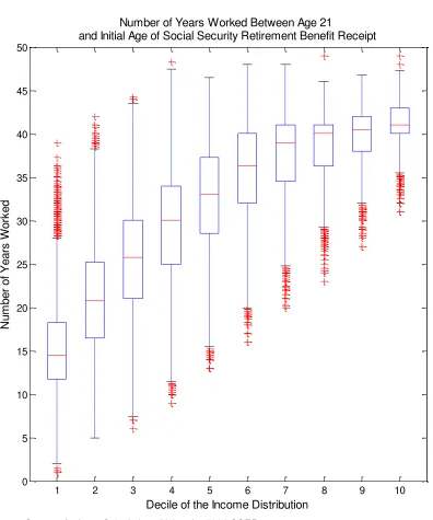
// Figure 4 About Here //
lifetime income distribution have worked at least 35 years. It is mostly in the upper deciles of the income distribution where we can find many people with long careers of at least 40 years. An implication for policy is that when reforms include minimum benefit guarantees for those with long careers, there will be few people who would meet the criteria for the guarantee. Again, however, we must include the possibility that some people who worked for shorter periods or who have low lifetime earnings may have spouses who acted as a primary earner, as was often the case for married women from these birth cohorts.
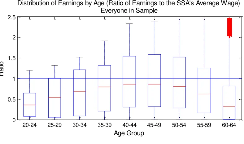
Patterns of Earnings by Age
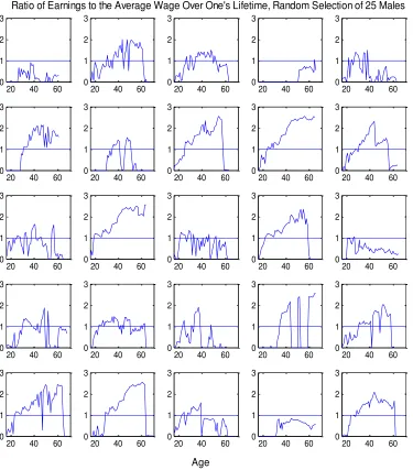
To begin, Figure 5 shows the lifetime earnings patterns for 25 randomly selected males, in which earnings at each age are reflected as the ratio of the worker’s earnings to the AWI of the corresponding year. Figure 6 repeats this exercise for females. In these figures, the hypothetical average worker’s earnings are reflected by the horizontal line at height one. This pattern does not apply to any actual workers, and indeed the figures show a great deal of diversity in worker earnings patterns. While the most common pattern shows a steady increase in relative earnings over time, a number of the cases show relative decreases over time and short careers. As for women, there are fewer cases of women earning the AWI level, and many women show temporary and sporadic attachments to the formal labor force.
// Figure 5 About Here //
// Figure 6 About Here //
Figures 7 and 8 quantify these matters more carefully by showing the distribution of earnings by age group. These figures demonstrate that the AWI overstates earnings by the most at early and older ages. In Figure 7, men and women are combined, and the inverse-U shape of earnings as one ages is clear. Earnings as a percentage of the AWI peak in a worker’s 40s. Nonetheless, the median earnings at any age group never reaches the level of the AWI, even when removing those who did not work in a particular five-year span, as is done in the bottom half of the figure. Figure 8 separates men and women, showing the age-earnings profile for each gender. For men, median earnings do exceed the AWI in the 30s, 40s, and early 50s, though they are less in the 20s and after age 55. Women, on the other hand, show strikingly lower
wages. Women’s peak earnings come in their late 40s and early 50s, but even at these ages,
more than 75 percent of the women who qualified for Social Security benefits on their own earnings records still did not earn at least the AWI.
// Figure 7 About Here //
The lower wages of women lead them to cluster in the lower lifetime income deciles. More than 80 percent of those in the lowest income deciles are women, while less than ten percent of the top income decile is women. Though many of these women may also be contributing to their household with nonsalaried work and may also be eligible for Social
not receiving a spousal benefit will be relatively worse off from any potential switch to individual accounts that do not include a redistribution component.
// Figure 8 About Here //
Asset Accumulations in Defined-Contribution Individual Accounts
We have observed a number of differences between hypothetical workers and actual workers, and now we investigate the implications for defined-contribution pensions, which are becoming an increasingly popular path for reform in countries dealing with aging populations. In the United States, the President’s Commission to Strengthen Social Security (2001) presented three proposals that would include personal retirement accounts (PRAs) as a part of Social
Security reform, and for about one year after President Bush’s re-election in 2004, America engaged in a serious debate about their potential merits. Likewise, Whitehouse (2007) cites the growth of mandatory defined-contribution pensions in countries ranging from Latin America and the Caribbean to Eastern Europe and Central Asia. This research can lend further insight to the issue, as we determine that the returns which could be expected for actual workers will tend to fall below their hypothetical counterparts on account of differences in both the shape and level of lifetime earnings. Here we quantify the differences and look for a hypothetical worker with characteristics that will better match the case of actual workers.
Matters here will be kept simple as we assume workers invest a fraction of their Social Security covered earnings into an individual account at the end of each year they work, and their assets will accumulate and grow with a constant annual nominal return of 8 percent. This rate of return is consistent with what is used by financial advisors to simulate savings growth, and it can be thought to imply a 3 percent inflation rate and a 5 percent real return. The choice of return is not particularly important, as we are mostly interested in differences between actual and
hypothetical workers sharing similar assumptions for their defined-contribution accounts, except that higher returns will create a bigger advantage for those with earnings early in their careers, which will therefore tend to produce even better results for hypothetical workers relative to actual workers.
// Table 4 About Here //
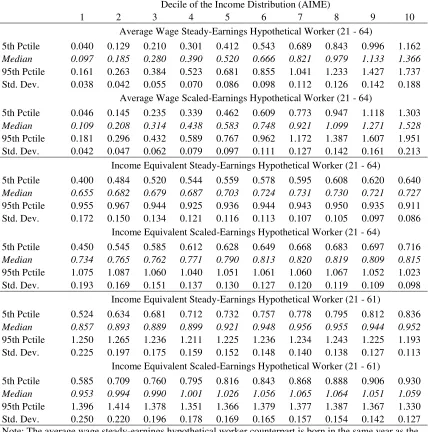
workers will indicate the role of earnings patterns in determining one’s portfolio accumulations. Finally, the fifth and sixth hypothetical workers are also income-equivalent workers, but they retire at age 62 rather than age 65.
For the table values, any number larger than one implies that the actual worker could obtain a higher benefit than their hypothetical counterpart, while values less than one imply that the hypothetical worker will do better. We express the results as ratios, because the actual levels of portfolio assets and benefits will depend on many factors, such as how much is saved, the actual returns to the accounts that can be achieved, whether annuitization is mandatory, the administrative and overhead costs from annuitization, the type of annuity is chosen, the
assumptions about asset returns and mortality for the annuity, and the transition costs that would be required to pay for promised benefits from the current Social Security system. It is the relative differences in outcomes for defined-contribution pensions between hypothetical workers and actual workers that interest us, and aside from emphasizing this important detail, the paper does not otherwise attempt to determine whether or not such reforms should be undertaken. We are interested to know what characteristics of actual workers lead them to do better relative to hypothetical workers, as well as what kind of hypothetical worker will be most comparable to actual workers.
First, Table 4 compares actual workers to the average wage steady-earnings hypothetical worker retiring at age 65. It is not until the 9th income decile that we find the median actual worker who can accumulate as much. In fact, workers in the bottom half of the income distribution can expect to retire with less than half the assets of the average wage hypothetical worker. For average wage scaled-earnings hypothetical workers who have less earnings in the early part of their careers, we find a closer connection to actual workers. Nonetheless, it is still not until the 8th income decile in which we find the median ratio to be larger than one. Both of these results suggest that the lifetime incomes of actual workers fall below hypothetical workers, and based on earnings levels, hypothetical workers will tend to overestimate the portfolio
accumulations of actual workers.
Next, the income-equivalent steady and scaled earnings workers allow us to examine the role of earnings patterns more directly after removing the impacts of earnings levels. With lifetime incomes adjusted to match each actual worker, the income-equivalent hypothetical workers will accumulate larger portfolios only when they have more earnings in the early parts of their careers compared to actual workers. Here we find clear evidence that standard
hypothetical worker.
Another important matter is that the standard deviations for the ratios decrease as we move up the income distribution, which suggests more volatility in the earnings patterns of low income workers. The 5th percentile ratio for low income workers is much lower than for high income workers, and even the 95th percentile is a little less. These results suggest a consistent effect in that low income workers do tend to obtain more of their earnings late in their careers, which puts them at a disadvantage in accumulating assets for their defined-contribution account. Studies using hypothetical workers will potentially make defined-contribution accounts look more favorable than may otherwise be possible.
Finally, Table 4 shows corresponding results when the hypothetical workers are assumed to retire at the early retirement age of 62. Actually, this assumption can move a long way toward alleviating the problems described before, particularly for the scaled-earnings worker. Though it is still the case that low wage workers will fare less well than high wage workers, the median ratios for the bottom decile is now 0.953, and by the fourth decile the median rises above one. This suggests, as a policy recommendation, that studies of defined-contribution pensions that use hypothetical workers should rely on scaled-earnings that can easily be obtained from a household survey that includes questions about age and wages in a given year, and should assume the earliest possible retirement age for the hypothetical worker.
CONCLUSIONS
References
Au, Andrew, Olivia S. Mitchell, John W.R. Phillips, 2004, Modeling Lifetime Earnings Paths: Hypothetical versus Actual Workers, Boettner Center for Pensions and Retirement Research, Working Paper No. BWP2004-3.
Bosworth, Barry, Gary Burtless, and C. Eugene Steuerle, 1999, Lifetime Earnings Patterns, the Distribution of Future Social Security Benefits, and the Impact of Pension Reform, Center for Retirement Research at Boston College, Working Paper 1999-06.
Caldwell, Steven, Melissa Favreault, Alla Gangman, Jagadeesh Gokhale, Thomas Johnson, and Laurence J. Kotlikoff, 1999, Social Security’s Treatment of Postwar Americans, in: James M. Poterba, ed., Tax Policy and the Economy, Vol. 13 (MIT Press, Cambridge, MA), 109-148.
Clingman, Michael, and Orlo Nichols, 2007, Scaled Factors for Hypothetical Earnings Examples Under the 2007 Trustees Report Assumptions, Actuarial Note (Office of the Chief Actuary, Social Security Administration) No. 2007.3.
Cohen, Lee, C. Eugene Steuerle, and Adam Carasso, 2001, Social Security Redistribution by Education, Race, and Income: How Much and Why, Paper for the Third Annual Conference of the Retirement Research Consortium.
Committee on Ways and Means of the US House of Representatives, 2004, Green Book (US House of Representatives, Washington, DC).
Coronado, Julia Lynn, Don Fullerton, and Thomas Glass, 1999, Distributional Impacts of Proposed Changes to the Social Security System, in: James M. Poterba, ed., Tax Policy and the Economy, Vol. 13 (MIT Press, Cambridge, MA), 149-186.
Fullerton, Don, and Brent Mast, 2005, Income Distribution from Social Security (American Enterprise Institute, Washington, DC).
Goss, Stephen C., and Alice H. Wade, 2002, Estimates of Financial Effects for Three Models Developed by the President’s Commission to Strengthen Social Security, Social Security Administration Memorandum.
Haider, Steven, and Gary Solon, 2006, Life-Cycle Variation in the Association Between Current and Lifetime Earnings, National Bureau of Economic Research Working Paper No. 11943.
Harris, Amy R., John Sabelhaus, and Jonathan A. Schwabish, 2006, Projecting Labor Force Participation and Earnings in CBO’s Long-Term Microsimulation Model, Congressional Budget Office Background Paper.
Hungerford, Thomas L., 2003, Do Workers with Low Lifetime Earnings Really Have Low Earnings Every Year?: Implications for Social Security Reform, The Levy Economics Institute of Bard College, mimeo.
Study of Socioeconomic Epidemiology, (Harvard University Press, Cambridge, MA).
Leimer, Dean R., 1995, A Guide to Social Security Money’s Worth Issues, Office of Research and Statistics (Social Security Administration) Working Paper No. 67.
Leimer, Dean R., 1999, Lifetime Redistribution Under the Social Security Program: A Literature Synopsis, Social Security Bulletin 62, No. 2, 1-9.
Nichols, Orlo R., Michael D. Clingman, and Milton P. Glanz, 2001, Internal Real Rates of Return Under the OASDI Program for Hypothetical Workers, Actuarial Note (Office of the Chief Actuary, Social Security Administration) No. 144.
Pfau, Wade D., 2003, Essays on Social Security Reform, unpublished Ph.D. dissertation, Department of Economics, Princeton University.
President’s Commission to Strengthen Social Security, 2001, Strengthening Social Security and Creating Personal Wealth for All Americans.
Smith, Karen, Eric Toder, and Howard Iams, 2001, Lifetime Distributional Effects of Social Security Retirement Benefits, Paper for the Third Annual Conference of the Retirement Research Consortium.
Steuerle, C. Eugene, and Jon M. Bakija, 1994, Retooling Social Security for the 21st Century: Right and Wrong Approaches to Reform (The Urban Institute Press, Washington, DC).
Steuerle, C. Eugene, Christopher Spiro, and Adam Carasso, 2000, Do Analysts Use Atypical Workers to Evaluate Social Security, Urban Institute Straight Talk on Social Security and Retirement Policy Series No. 19.
Toder, Eric, Lawrence Thompson, Favreault, Richard Johnson, Kevin Perese, Caroline Ratcliffe, Karen Smith, Cori Uccello, Timothy Waidmann, Jillian Berk, Romina Woldemariam, Gary Burtless, Claudia Sahm, and Douglas Wolf, 2002, Modeling Income in the Near Term: Revised Projections of Retirement Income through 2020 for the 1931-1960 Birth Cohorts (The Urban Institute, Washington, DC).
TABLE 1
Datasets With Earnings Used in United States Social Security Studies
Name of Dataset Details About Data
Links to Social Security Earnings Records (SSER) SSA Benefits and Earnings
Public-Use File Provides Annual Social Security Covered Earnings Data since 1951 This is the SSER data
Survey of Income and Program Participation (SIPP)
U.S. Census Bureau survey is meant to provide information to the government about the effectiveness of its social programs. Survey has continued since 1984 with a series of panels lasting 2.5 to 4 years each
Yes, can be linked
Health and Retirement Survey (HRS)
University of Michigan survey of about 22,000 individuals aged 50 and over in 1998. Survey is longitudinal and is conducted every two years since 1992
Yes, can be linked
Panel Study of Income Dynamics (PSID)
Panel data for 8,000 families since 1968. After the 2003 updates, the survey included information for up to 36 years in the lives of 65,000 individuals.
No direct link, but statistical matching techniques have been used
Current Population Survey (CPS)
U.S. Government survey includes earnings data with its annual March survey. It provides cross-section data for United States workers, but no panel data links are available between years.
TABLE 2
The Distribution of Top-coded Earnings By Income Level
Decile of the Income Distribution
Number of Years of Topcoded Earnings
0 1 - 5 6 - 10 11 - 20 21 + Row Totals
1 9.93% 0.07% 0% 0% 0% 10% 2 9.48% 0.52% 0% 0% 0% 10% 3 8.78% 1.18% 0.04% 0% 0% 10% 4 7.91% 1.84% 0.24% 0.01% 0% 10% 5 6.51% 2.64% 0.69% 0.16% 0% 10% 6 4.55% 3.25% 1.41% 0.77% 0.01% 10% 7 2.15% 3.47% 2.06% 2.10% 0.23% 10% 8 0.53% 2.16% 2.41% 3.75% 1.15% 10% 9 0.04% 0.63% 1.44% 4.37% 3.51% 10% 10 0% 0.04% 0.26% 1.97% 7.73% 10%
[image:19.612.93.518.136.570.2]Column Totals 49.88% 15.80% 8.55% 13.13% 12.63%
TABLE 3
Distribution of Current Income for those Aged 62 to 71, Based on Social Security Beneficiary Status
Not Receiving Social Security
TABLE 4
Ratio of Worker's Total Portfolio at Retirement to Hypothetical Worker Counterpart's Portfolio
Decile of the Income Distribution (AIME)
1 2 3 4 5 6 7 8 9 10
Average Wage Steady-Earnings Hypothetical Worker (21 - 64)
5th Pctile 0.040 0.129 0.210 0.301 0.412 0.543 0.689 0.843 0.996 1.162
Median 0.097 0.185 0.280 0.390 0.520 0.666 0.821 0.979 1.133 1.366
95th Pctile 0.161 0.263 0.384 0.523 0.681 0.855 1.041 1.233 1.427 1.737 Std. Dev. 0.038 0.042 0.055 0.070 0.086 0.098 0.112 0.126 0.142 0.188
Average Wage Scaled-Earnings Hypothetical Worker (21 - 64)
5th Pctile 0.046 0.145 0.235 0.339 0.462 0.609 0.773 0.947 1.118 1.303
Median 0.109 0.208 0.314 0.438 0.583 0.748 0.921 1.099 1.271 1.528
95th Pctile 0.181 0.296 0.432 0.589 0.767 0.962 1.172 1.387 1.607 1.951 Std. Dev. 0.042 0.047 0.062 0.079 0.097 0.111 0.127 0.142 0.161 0.213 Income Equivalent Steady-Earnings Hypothetical Worker (21 - 64)
5th Pctile 0.400 0.484 0.520 0.544 0.559 0.578 0.595 0.608 0.620 0.640
Median 0.655 0.682 0.679 0.687 0.703 0.724 0.731 0.730 0.721 0.727
95th Pctile 0.955 0.967 0.944 0.925 0.936 0.944 0.943 0.950 0.935 0.911 Std. Dev. 0.172 0.150 0.134 0.121 0.116 0.113 0.107 0.105 0.097 0.086
Income Equivalent Scaled-Earnings Hypothetical Worker (21 - 64)
5th Pctile 0.450 0.545 0.585 0.612 0.628 0.649 0.668 0.683 0.697 0.716
Median 0.734 0.765 0.762 0.771 0.790 0.813 0.820 0.819 0.809 0.815
95th Pctile 1.075 1.087 1.060 1.040 1.051 1.061 1.060 1.067 1.052 1.023 Std. Dev. 0.193 0.169 0.151 0.137 0.130 0.127 0.120 0.119 0.109 0.098 Income Equivalent Steady-Earnings Hypothetical Worker (21 - 61)
5th Pctile 0.524 0.634 0.681 0.712 0.732 0.757 0.778 0.795 0.812 0.836
Median 0.857 0.893 0.889 0.899 0.921 0.948 0.956 0.955 0.944 0.952
95th Pctile 1.250 1.265 1.236 1.211 1.225 1.236 1.234 1.243 1.225 1.193 Std. Dev. 0.225 0.197 0.175 0.159 0.152 0.148 0.140 0.138 0.127 0.113
Income Equivalent Scaled-Earnings Hypothetical Worker (21 - 61)
5th Pctile 0.585 0.709 0.760 0.795 0.816 0.843 0.868 0.888 0.906 0.930
Median 0.953 0.994 0.990 1.001 1.026 1.056 1.065 1.064 1.051 1.059
95th Pctile 1.396 1.414 1.378 1.351 1.366 1.379 1.377 1.387 1.367 1.330 Std. Dev. 0.250 0.220 0.196 0.178 0.169 0.165 0.157 0.154 0.142 0.127 Note: The average wage steady-earnings hypothetical worker counterpart is born in the same year as the worker and earns the Average Wage Index for each age of employment (indicated in parenthesis). The scaled-earnings worker is the same as the steady-earnings worker, except that lifetime earnings are rescaled to show the inverted-U shape earnings pattern provided in Clingman and Nichols (2007). Income-Equivalent counterpart workers have their incomes adjusted up or down so that they have the same AIME as each worker in the sample.
Figure 1
1955 1960 1965 1970 1975 1980 1985 1990 1995 2000 1
1.5 2 2.5
Ratio of the Maximum Taxable Wage to the Average Wage Index, 1951-2003
1955 1960 1965 1970 1975 1980 1985 1990 1995 2000 0
5 10 15 20 25 30 35
Percent of Workers At Maximum Taxable Wage, 1951-2003
Figure 2
1 2 3 4 5 6 7 8 9 10
62 63 64 65 66 67 68 69 70
Ag
e
o
f
So
c
ia
l Se
c
u
ri
ty
R
e
tire
m
e
n
t
Be
n
e
fit
U
p
ta
k
e
Initial Age of Social Security Retirement Benefit Receipt Across the Income Distribution
Decile of the Income Distribution Source: Author's Calculations Using the 2004 SSER
Figure 3
0 10 20 30 40 50 60 70 80 90 100 0
5 10 15 20 25 30 35 40 45 50
Number of Years Worked Between Age 21
and Initial Age of Social Security Retirement Benefit Receipt
Percentage of Sample
N
u
m
b
e
r
o
f
Ye
a
rs
W
o
rk
e
d
Males Females Aggregate
Figure 4
1 2 3 4 5 6 7 8 9 10
0 5 10 15 20 25 30 35 40 45 50
N
u
m
b
e
r
o
f
Ye
a
rs
W
o
rk
e
d
Number of Years Worked Between Age 21
and Initial Age of Social Security Retirement Benefit Receipt
Decile of the Income Distribution Source: Author's Calculations Using the 2004 SSER
Figure 5
20 40 60 0
1 2 3
20 40 60 0
1 2 3
20 40 60 0
1 2 3
20 40 60 0
1 2 3
20 40 60 0
1 2 3
20 40 60 0
1 2 3
20 40 60 0
1 2 3
20 40 60 0
1 2 3
20 40 60 0
1 2 3
20 40 60 0
1 2 3
20 40 60 0
1 2 3
20 40 60 0
1 2 3
20 40 60 0
1 2 3
20 40 60 0
1 2 3
20 40 60 0
1 2 3
20 40 60 0
1 2 3
20 40 60 0
1 2 3
20 40 60 0
1 2 3
20 40 60 0
1 2 3
20 40 60 0
1 2 3
20 40 60 0
1 2 3
20 40 60 0
1 2 3
20 40 60 0
1 2 3
20 40 60 0
1 2 3
20 40 60 0
1 2 3
Ratio of Earnings to the Average Wage Over One's Lifetime, Random Selection of 25 Males
Age
Figure 6
20 40 60 0
1 2 3
20 40 60 0
1 2 3
20 40 60 0
1 2 3
20 40 60 0
1 2 3
20 40 60 0
1 2 3
20 40 60 0
1 2 3
20 40 60 0
1 2 3
20 40 60 0
1 2 3
20 40 60 0
1 2 3
20 40 60 0
1 2 3
20 40 60 0
1 2 3
20 40 60 0
1 2 3
20 40 60 0
1 2 3
20 40 60 0
1 2 3
20 40 60 0
1 2 3
20 40 60 0
1 2 3
20 40 60 0
1 2 3
20 40 60 0
1 2 3
20 40 60 0
1 2 3
20 40 60 0
1 2 3
20 40 60 0
1 2 3
20 40 60 0
1 2 3
20 40 60 0
1 2 3
20 40 60 0
1 2 3
20 40 60 0
1 2 3
Ratio of Earnings to the Average Wage Over One's Lifetime, Random Selection of 25 Females
Age
Figure 7
20-24 25-29 30-34 35-39 40-44 45-49 50-54 55-59 60-64 0
0.5 1 1.5 2 2.5
R
a
tio
Age Group
Distribution of Earnings by Age (Ratio of Earnings to the SSA's Average Wage) Everyone in Sample
20-24 25-29 30-34 35-39 40-44 45-49 50-54 55-59 60-64 0
0.5 1 1.5 2 2.5
R
a
tio
Age Group
Distribution of Earnings by Age (Ratio of Earnings to the SSA's Average Wage) Conditional on Working at Some Point in Each Age Range
Figure 8
20-24 25-29 30-34 35-39 40-44 45-49 50-54 55-59 60-64 0
0.5 1 1.5 2 2.5
R
a
tio
Age Group
Distribution of Earnings by Age (Ratio of Earnings to the SSA's Average Wage) All Males in Sample
20-24 25-29 30-34 35-39 40-44 45-49 50-54 55-59 60-64 0
0.5 1 1.5 2 2.5
R
a
tio
Age Group
Distribution of Earnings by Age (Ratio of Earnings to the SSA's Average Wage) All Females in Sample