MEASURING PROCESS INNOVATION ON DOUBLE FLANKED CONCEPTUAL MODEL FOR KNOWLEDGE SHARING ON ONLINE LEARNING ENVIRONMENT

1524

LONG-TERM DEEP LEARNING LOAD FORECASTING

BASED ON SOCIAL AND ECONOMIC FACTORS IN THE

KUWAIT REGION

1_{SALMAN ZAKARYA,} 2_{HALA ABBAS,} 3_{MOHAMMED BELAL}

Helwan University, Faculty of Computers & Information, Department of Computer Science, Cairo, Egypt

1_s

[email protected], [email protected], [email protected]

ABSTRACT

Load forecasting (LF) is a technique used by energy-providing companies to predict the power needed. LF is of great importance for ensuring sufficient capacity and manipulating the deregulation of the power industry in many countries, such as Arab gulf countries. Moreover, reduction of load forecasting error leads to lower costs and could save billions of dollars. Recently, further improvement has been introduced using more complex models that take into account dependencies among hidden layers. Also, many approach based model are presented, but all of them have limitations prediction capabilities. The purpose of this work is to demonstrate the load forecasting classes and factors impacting its performance, especially in Kuwaiti region in Arab Gulf. This work presents a novel deep leaning model that involves generating more accurate predictions for the electric load based on hierarchal learning architecture. It is integrates the features of data in discovering most influent factors affecting electrical load usage. The dataset used is the actual data from Ministry of Electrical in Kuwait, the data for load is in mega-watt long-term for the years 2006 to year 2015, which is trained using ARIMA and neural networks models. The load forecasting is done for the year 2016 and is validated for the accuracy and less for error rate. Results indicate that this architecture performs quite well when compared to traditional approaches and deep neural network.

Keywords: Power Electricity; Load forecasting; ARIMA; Regression; Long-term; Prediction; deep learning;

1. INTRODUCTION

Forecasting is the process of estimating the qualitative or quantitative future data by means of calculation. Forecasting has been applied in many areas and it is sometimes human driven due to its complexity. It could be considered one of the most difficult tasks because of the uncertainty about the

future [1]. Load forecasting is a technique used by

energy-providing companies to predict the

power/energy needed to meet the demand and supply equilibrium. Its importance in business, economics, government, and many other fields, and guide many important decisions [2]. Therefore, good forecasts help to produce good decisions such as decisions on purchasing and generating electric

power, load switching, and infrastructure

development [3].

Basically, an electric load refers to the power consumed by an electric circuit at its output terminal [5]. In other words, load forecasting is

way of estimating what future electric load will be for a given forecast horizon based on the available information about the state of the system [6]. In addition, forecasting is inextricably linked to building statistical models before forecast a variable of interest, also, build a model and estimate the model's parameters using observed

historical data. Typically, estimated model

summarizes dynamic patterns in the data [6], which

is estimates model provides a statistical

characterization of the links between the present and the past data.

1525 important differences in load between weekdays and weekend [6] [8]. For example, Mondays and Fridays being adjacent to weekends, may have structurally different loads than Tuesday through Thursday.

On the other hand, Deep Learning (DL) is a new area of Machine Learning research, which has been introduced with the objective of moving Machine Learning closer to one of its original goals: Artificial Intelligence. DL allows computational models that are composed of multiple processing layers to learn representations of data with multiple levels of abstraction.

In other hand, forecasts can also be classified based on the forecasting horizon. A common classification of load forecasting used in [17], as the following [18]:

•Very Short-Term Load Forecasting (VSTLF): A

forecasting horizon of under 1 hour;

•Short-Term Load Forecasting (STLF): A

forecasting horizon of under one week;

•Medium-Term Load Forecasting (MTLF): A

forecasting horizon of under 1 year; and

•Long-Term Load Forecasting (LTLF): A

forecasting horizon of over 1 year. Table 1 shows taxonomy of load forecasting.

Table 1:Taxonomy of Load Forecasting [16] Load Forecast Period Importance

Long 1-10

Years

To calculate and to allocate the required future capacity. To plan for new power station to

face customer

requirements

Plays an essential role to determine future budget.

Medium 1-week

to few months

Fuel allocation and maintenance schedules Accurate for power system operation.

Short 1-hour to

1-week

To evaluate economic dispatch, hydro-thermal co-ordination, unit commitment, transaction. To analysis system security among other mandatory function. Very-Short 1-minite

-1-hour

Energy management system(EMS)

Time series prediction can be divided into two categories depending on prediction time period: short term and long term [18]. The forecasting algorithms aim to forecast future values based on the present and historical data. The tools for prediction include: neural networks, regression, Support Vector Machine (SVM), and discriminate

analysis. Recently, data mining techniques such as neural networks, fuzzy logic systems, genetic algorithms and rough set theory are used to predict control and failure detection tasks [5]. Most forecast use statistical techniques or artificial intelligence algorithms such as regression, neural networks, fuzzy logic, and expert systems. For example, Chen et al. [4] presented an additive model that takes the form of predicting load as the function of four components:

L = Ln + LW + Ls + Lr

where L is the total load, Ln represents the “normal” part of the load, which is a set of standardized load shapes for each “type” of day that has been identified as occurring throughout the year, Lw represents the weather sensitive part of the load, Ls is a special event component that create a substantial deviation from the usual load pattern, and Lr is a completely random term the noise.

1.1.The forecasting method and techniques Based on the relation with external factors, load forecasting models can be classified into two categories: time-of-day models and dynamic models. Parametric load forecasting methods can be implemented using regression methods, time series prediction methods. For decades, time series have been used in fields such as economics, digital signal processing as well as electric load forecasting.

Models of time series include ARIMA

(autoregressive integrated moving average) and

ARIMAX (autoregressive integrated moving

average with exogenous variables).

a) Statistical model-based learning: The end-use and econometric methods require a large amount of information relevant to appliances, customers, economics, etc. In order to simplify the medium-term forecasts, make them more accurate, and avoid the use of the

unavailable information, the following

multiplicative model is the most accurate as shows in equation1.

L (t) = F (d (t), h (t)) – f (w (t)) + R (t) (1)

where L(t) is the actual load at time t, d(t) is the day of the week, h(t) is the hour of the day, F(d, h) is the daily and hourly component, w(t) is the weather data that include the temperature and humidity, f(w) is the weather factor, and R(t) is a random error.

1526

ᵝ ∑ ᵝ

(2)

where Xj are explanatory variables which are nonlinear functions of current and past weather parameters and β0, βj are the regression coefficients.

b) Time Series: Time Series Analysis Regression

techniques were combined with ARIMA models. Regression techniques were used to model and forecast the peak and trough load. Then ARIMA was applied to a weather normalized load to produce the forecast. Time series methods are based on the assumption that the data have an internal structure, such as autocorrelation, trend, or seasonal variation.

c) Regression methods: Regression is the one of

most widely used statistical techniques. For electric load forecasting regression, methods are usually used to model the relationship of load consumption and other factors such as weather, day type, and customer class.

d) Neural Networks (NN): The have been a widely

studied electric load forecasting technique since 1990. Neural networks are essentially non-linear circuits that have the demonstrated capability to do non-linear curve fitting. The outputs of an artificial neural network are some linear or nonlinear mathematical function of its inputs. The inputs may be the outputs of other network elements as well as actual network inputs. The

most popular artificial neural network

architecture for electric load forecasting is back

propagation. Back propagation neural networks use continuously valued functions and supervised learning. The under supervised learning, actual numerical weights assigned to element inputs are determined by matching historical data (such as time and weather) to desired outputs (such as historical electric loads) in a pre-operational “training session”.

e) Support Vector Machine (SVM) is a more

recent powerful technique for solving

classification and regression problems. This approach was originated from statistical learning theory. Unlike neural networks, which try to define complex functions of the input feature space, support vector machines perform a nonlinear mapping (by using so-called kernel functions) of the data into a high dimensional (feature) space. Support vector machines use simple linear functions to create linear decision boundaries in the new space. Mohandes [3] applied support vector machines for short-term electrical load forecasting. Chen et al. [2]

proposed a SVM model to predict daily load demand of a month.

Many researchers in the load forecasting models in the electric power system based approach presented such as in machine learning techniques (SVM, NN, etc.) but all of them have limitations prediction capabilities. Therefore, the problem of forecasting the electrical load in Kuwait and Arab Gulf has become crucial and critical in the recent years. The increasing and fluctuating load consumption has led to several problems such as occasional network power fault and failure.

In this paper, a soft computing based deep

learning model is introduced, its integrate the features of data in discovering the most influent factors affecting electrical load usage, and their interrelations as well as the power of linear regression and neural networks to approximate the load forecasting in order to introduce a model for load forecasting that takes into consideration the actual factors that affects the electrical usage. While the long term used in this approach. The dataset used in this paper is for the Kuwait Electricity Authority of DC Network for the last 10 years as long term taxonomy.

The rest of this paper is organized as follow: Section 2 presents the Related Work briefly.

Section 3 describes the proposed model

Architecture and methodology. Section 4 shows the experimental results and discussions. The paper is concluded in section 5.

2. RELATED WORK

Forecasting is a planning tool that helps management in its attempts to cope with the uncertainty of the future, relying mainly on data from the past and present, also analysis of trends [2]. Therefore, extracting the relevant information from the huge amount of data is highly complex, costly, and time consuming. This complex problem requires to using soft computing techniques to cope with large number of factors for the actual power generation needed. This section present briefly the researches for prediction load forecasting from three aspects: the techniques developed, the representative work done, and viruses parameter deployed.

A novel applied approach to data analysis for power system based on data mining theory presented in research [2], the authors develop new

application to analysis data for electrical

1527 information processing, pattern recognition and artificial intelligence etc.

In the load forecasting power system, the time-series factors include the time of the year, the day of the week, and the hour of the day. There are important differences in load between weekdays and weekends. The load on different weekdays also can behave differently [6] [8].

Numerous methods and clustering algorithms have been planned previous to support clustering of time series data streams [4]. The paper [7], present a pragmatic methodology that can be used as a guide to construct Electric Power Load Forecasting models. This methodology is mainly based on decomposition and segmentation of the load time series. In his work, Azadeh et al as [25] have proposed an integrated fuzzy system, data mining and time series framework to estimate and predict electricity demand for seasonal and monthly changes in electricity consumption especially in developing countries such as China and Iran with non-stationary data. In [20] proposed an algorithm using an unsupervised/supervised learning concept and historical relationship between the load and temperature for a given season, day type and hour of the day. They used this algorithm to forecast hourly electric load with a lead time of 24 hrs.

In recent years, many deep learning methods have been shown to achieve state-of-the-art performance in many research areas: speech recognition [10], computer vision [23] and natural language processing [15]. This promise has not been demonstrated in other areas of computer science due to a lack of thorough research.

In addition, forecasting is predicting unknown or future values of other variables. It’s achieved by

subjecting a huge amount of data to a training rule known as supervised learning, by estimated values are compared with known results [19]. In the same aspect, a new type of data mining based on data analysis load forecasting and the fast diagnostic reasoning algorithm presented in the research [3], it has obvious advantages in dealing with a large number of power system data, the data were analyzed by a logical of the relevance degree. The authors combine data mining algorithms and the system improves state analysis and mining. They are conclude that the approach provide a great deal of information for aid decision making for planning and designing new electric power for enterprises.

Research [4] presents an overview of data mining techniques used in power systems. In his paper Azadeh et al. [25] proposed an integrated fuzzy system for data mining and time series framework to estimate and predict electricity demand for seasonal and monthly changes in electricity consumption especially in developing countries such as China and Iran with non-stationary data.

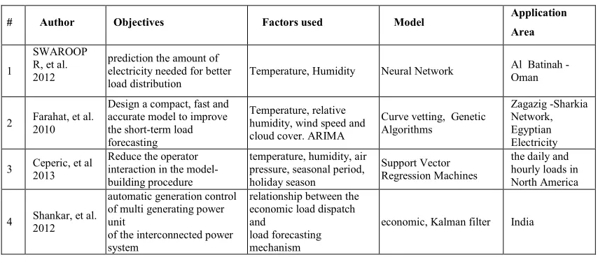
Table 2 shows the load forecasting approaches based Factors which are used.

Based on the previous works, many researchers worked in prediction load forecasting, and a lot of models for the electric power system based approach where presented such as in machine learning techniques (SVM, NN, etc.), but all of them have limitations prediction capabilities.

Therefore, the problem of forecasting the electrical load in Kuwait and Arab Gulf has become crucial and critical in the recent years. The increasing and fluctuating load consumption has led to several problems such as occasional network

power fault and failure.

Table 2: Load Forecasting Approaches based Factors

# Author Objectives Factors used Model Application

Area

1

SWAROOP R, et al. 2012

prediction the amount of electricity needed for better load distribution

Temperature, Humidity Neural Network Al Batinah - Oman

2 Farahat, et al. 2010

Design a compact, fast and accurate model to improve the short-term load forecasting

Temperature, relative humidity, wind speed and cloud cover. ARIMA

Curve vetting, Genetic Algorithms

Zagazig -Sharkia Network, Egyptian Electricity

3 Ceperic, et al ₂₀₁₃

Reduce the operator interaction in the model-building procedure

temperature, humidity, air pressure, seasonal period, holiday season

Support Vector Regression Machines

the daily and hourly loads in North America

4 Shankar, et al. 2012

automatic generation control of multi generating power unit

of the interconnected power system

relationship between the economic load dispatch and

load forecasting mechanism

1528

5 Stojanovi´c, et al.2010

Predict maximum daily load for period of one month, using different data sets and features

Maximum daily load for past seven days • Average daily temperatures (T), • Day Of the Week (D).

SVM

Eastern Slovakian Electricity Corporation for the EUNITE competition

6 Hinojosa, et al. 2011

apply fuzzy inductive reasoning (FIR) for Short-Term Load Forecasting in power systems

Weather and load) and qualitative variables (day, season, etc.)

ANN, fuzzy inductive reasoning (FIR)

Ecuadorian Energy Market

7 Guan, et al ₂₀₁₃ Very short-term load _forecasting Filter Wavelet Transform neural networks ISO New _England.

8 Woo-Joo Lee et al. 2015

forecasting the electric power load, mid term

air temperature

dependency of power load fuzzy time series

Seoul metropolitan area

9 Hong, Tao, 2014

Enhance and defensible forecasts, long term

Predictive modeling, scenario analysis, and weather normalization

multiple

linear regression models,

North Carolina Electric Membership Corporation

10 Riswan et al. 2015

daily forecasting of Malaysian electricity

Linguistic out-sample forecast by using the index numbers of linguistics approach.

fuzzy logical relationships

Malaysian electricity

11 Shu Fan, et al.2010

Prediction, semi-parametric additive models

Calendar variables, lagged actual demand

observations, historical and forecast temperature traces.

Artificial Neural

Network Australia

12 Ming-Yue Zhai2015

Load forecasting based on fractal interpolation, short term

Self-similarity theory and fractal interpolation. wavelet analysis

Parameter estimation fractal interpolation and fractal extrapolation

Shanxi Province

13 X. Song 2006

new hybrid short-term load forecasting

algorithm

temperature during spring, fall, and winter seasons is small

fuzzy linear regression method and general exponential smoothing

South Korea

3. THE PROPOSED SOFT COMPUTING

MODEL BASED LONG-TERM FOR LOAD FORECASTING

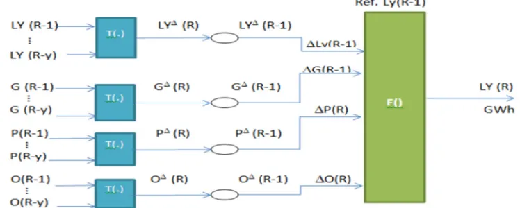
Figure 1 show proposed long-term model for the load forecasting prediction architecture. The model

consists of the most factors used based learning, which are: previous load in megawatt, Gross Domestic, Population, and Oil-price.

Ly: Electricity Load (GWh) in a Year, G: Gross domestic predict, P: Population, O: Oil price, Ref. energy: Reference.

1529

Figure 1: The proposed long term model Architecture

a. Dataset

The dataset used in this paper is the actual data from Ministry of Electrical in the Kuwait. The dataset is for 10 years from (2006 to 2015), its yearly details for a set of electricity and social factors in the Golf Area (Kuwait), which are listed

in the following: Factors for Load Forecast: the real

electrical loads are partial by a variety of factors. In this section, we study some of the most important factors. On the basis of these analyses, we consider extracting representative features which are used as

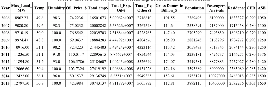
input of our deep model for load prediction. We focus in this paper on load periodicity, time dependency, weather influence (temperature and humidity), Oil_price, Gross Domestic, Population, Passengers, Residence, Currency Earning Rate, Average Salary, and economic factors like (total import and export in USD). In the following, table 3 shows the list of all factors that are collected and under goes to forecast and predict with a sample data. While the figure 3 shows the time series trend for the sample factors.

Table 3: List of Data for the load forecasting, Economic and Social Factors

Year Max_Load_

MW Temp. Humidity Oil_Price_$ Total_imp$

Total_Exp. Oil-$

Total_Exp Others$

Gross Domestic

Billion_$ Population

Passengers-Arrivals Residence CER ASE

2006 8962.23 49.6 98.3 74.2236 16501673 5.09062e+007 2716610 101.55 2389498 6100000 1633327 0.290 1050

2007 9080.80 49.6 98.3 75.0232 20002848 5.53626e+007 3267548 114.64 2538591 7137000 1715458 0.280 1100

2008 9710.19 50.0 100.0 76.8542 22039703 7.31884e+007 4228765 147.40 2705290 7493850 1806210 0.270 1100

2009 9974.47 48.8 100.0 69.0437 18884283 4.44792e+007 4804576 105.90 2881243 8168296 1934272 0.290 1250

2010 10916.00 51.1 90.2 82.4223 21445403 5.49424e+007 4323116 115.42 3059473 8513345 2084144 0.290 1250

2011 11236.50 51.1 91.0 110.0117 22895615 8.8667e+007 4854544 154.03 3239181 8426737 2166275 0.280 1376

2012 11894.80 51.2 93.0 106.5786 25184607 1.00243e+008 5526649 174.07 3419581 8877883 2257027 0.280 1420

2013 12066.60 50.4 100.0 103.7324 27419192 1.00668e+008 6131228 174.16 3593689 8000000 2385089 0.285 1420

2014 12422.00 56.1 96.0 80.1537 29136749 8.8551e+007 5949385 153.61 3753121 10027000 2468018 0.285 1500

2015 12797.50 50.8 100.0 42.3984 30743137 4.81188e+007 5605872 112.81 3892115 10400000 2592276 0.303 1650

Figure 4 shows the methodology for proposed long

term load forecasting model. The model

architecture consists of five modules which are: Historical Load for Previous Years, weather previous,

Model Forecaster, Load forecast, other factor forecast Time series forecasting, and Load forecasting predict (MW).

The data under goes into two main processes: time-series forecasting and prediction step.

1) Time-series forecast (TSF): every factor in

dataset goes into time-series forecasting analysis, the algorithm used is ARIMA as shows in the following:

Given a time series of data Xt where t is an integer index and the Xt are real numbers, an ARMA (p, q) model is given by equivalently (3).

(3)

where L is the lag operator, the ἁ are the parameters of the autoregressive part of the model, the ᶿ are the parameters of the moving average part and the ɛ are error terms. The error terms are generally assumed to be independent, identically distributed variables sampled from a normal distribution with zero mean.

2) Moving modeling in prediction: in this step, we

1530

Figure 3: Time series trend for the factors used

Figure 4: Methodology for proposed long term forecasting model

4. EXPERIMENTAL RESULTS AND

DISCURSIONS

The proposed long-term load forecasting based approach has designed and implemented using the

gretl1_tool. In the experimental results the time

series forecasting and regression forecasting is applied. The gretl_tool is used. Gretl is a cross-platform software package for econometric analysis, Gnu Regression, Econometrics and Time-series Library. It is free, open-source software. There is a lot of forecasting model based regression in gretl_tool, which is used in the experiments. The best one for regression model used as in the follow:

1

http://gretl.sourceforge.net/

a) Training the model forecasting using the actual

data for long-term 10-years from (2006-2015). Model: OLSR, using observations 2006-2015

(T = 10), Dependent variable: Load_MW.

Table 4: OLSR model forecasting

Factors Coefficient Std. Error t-ratio p-value

weather_temp. 38.1776 79.1167 0.4825 0.6624 Oil_price 4.94241 7.32786 0.6745 0.5483 Gross_Domestic_Billion 8.83792 18.7439 0.4715 0.6694 Population −0.00144 0.00838 −0.1728 0.8738 CER_1KD_1USD 30026.9 45957.3 0.6534 0.5601 ASE_monthly_KD −0.04242 2.61026 −0.0163 0.9881 Time 619.737 1226.6 0.5052 0.6482

Figure 4: Load Megawatt Polynomial Trends

8000 8500 9000 9500 10000 10500 11000 11500 12000 12500 13000

2007 2009 2011 2013 2015 Load_MW 46 48 50 52 54 56 58 60

2007 2009 2011 2013 2015 weather_tp 30 40 50 60 70 80 90 100 110 120

2007 2009 2011 2013 2015 oil_pric 4e+007 5e+007 6e+007 7e+007 8e+007 9e+007 1e+008 1.1e+008

2007 2009 2011 2013 2015 total_expOil 90 100 110 120 130 140 150 160 170 180

2007 2009 2011 2013 2015 Gross_Domestic_Billion

2.2e+006 2.4e+006 2.6e+006 2.8e+006 3e+006 3.2e+006 3.4e+006 3.6e+006 3.8e+006 4e+006

2007 2009 2011 2013 2015 Popolation

5.5e+006 6e+006 6.5e+006 7e+006 7.5e+006 8e+006 8.5e+006 9e+006 9.5e+006 1e+007 1.05e+007 1.1e+007

2007 2009 2011 2013 2015 Passengers_Arraivals 1.4e+006 1.6e+006 1.8e+006 2e+006 2.2e+006 2.4e+006 2.6e+006 2.8e+006

2007 2009 2011 2013 2015 Residenices 1000 1100 1200 1300 1400 1500 1600 1700

2007 2009 2011 2013 2015 ASE_monthly_KD 8000 8500 9000 9500 10000 10500 11000 11500 12000 12500 13000

2006 2007 2008 2009 2010 2011 2012 2013 2014 2015 2016

L o a d m w -P o ly n o m ia l t r e n d Years Load_MW (original data)

1531

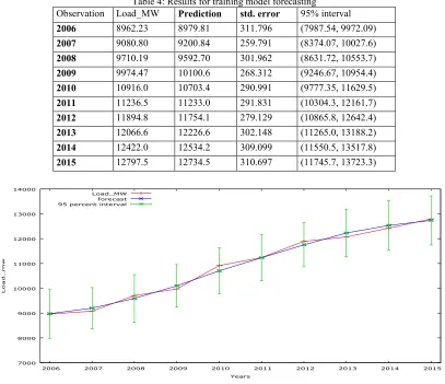
Table 4: Results for training model forecasting Observation Load_MW Prediction std. error 95% interval

2006 8962.23 8979.81 311.796 (7987.54, 9972.09)

2007 9080.80 9200.84 259.791 (8374.07, 10027.6)

2008 9710.19 9592.70 301.962 (8631.72, 10553.7)

2009 9974.47 10100.6 268.312 (9246.67, 10954.4)

2010 10916.0 10703.4 290.991 (9777.35, 11629.5)

2011 11236.5 11233.0 291.831 (10304.3, 12161.7)

2012 11894.8 11754.1 279.129 (10865.8, 12642.4)

2013 12066.6 12226.6 302.148 (11265.0, 13188.2)

2014 12422.0 12534.2 309.099 (11550.5, 13517.8)

2015 12797.5 12734.5 310.697 (11745.7, 13723.3)

Figure 5: load Forecasting for years (2006-2015)

b) Load forecasting for the new year: after the

training the model and approved the valid forecasting with near to the actual data, the load forecasting is done for new year as show in Table 5, which applied by using the regression

model as shown in the follow: Regression without Time Series Model: Forecasting new year using OLS Regression for year from (2006-2015).

Table 5: Testing model forecasting for 95% confidence intervals, t (4, 0.025) = 2.776

Obs. Load_MW prediction std.

error 95%interval

2006 8962.23 8988.23 2007 9080.8 9432.55 2008 9710.19 9492.72 2009 9974.47 10011.47

2010 10916 10527.59

2011 11236.5 11508.65

2012 11894.8 11626.78

2013 12066.6 12249.68

2014 12422 12438.61

2015 12797.5 12985.23 577.44 11382-14588.5

2016 13637.4 1027.84 10283.9-16990.9

7000 8000 9000 10000 11000 12000 13000 14000

2006 2007 2008 2009 2010 2011 2012 2013 2014 2015

L

o

a

d

_

m

w

Years Load_MW

1532 Forecast evaluation statistics:

Mean Error -187.73 Mean Squared Error 35244 Root Mean Squared Error 187.73 Mean Absolute Error 187.73

Table 6: comparison for load_MW based factor (Population)

OLS, using observations 2006-2015 (T = 10) Dependent variable: Load_MW

Coefficient Std. Error t-ratio p-value

const 2455.1 362.681 6.7693 0.0001

Population 0.00268527 0.000113856 23.5847 <0.0001

VAR system, lag order 1 Equation 1: Load_MW

Coefficient Std. Error t-ratio p-value

const 2776.82 888.203 3.1263 0.0204

Popolation 0.00344778 0.00116105 2.9695 0.0250

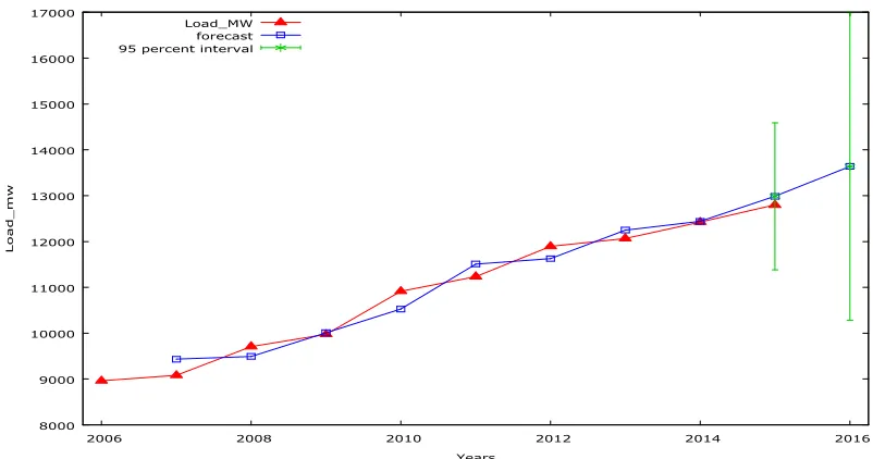
Figure 6: Load forecast for actual years (2006-2015) and forecast load curve for year 2016

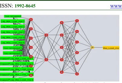
c) Forecasting using neural network (nn) model

In this experiment the nn implemented, the number of hidden layers used are HL=2 with 5 nodes, and HL=3 with 10 nodes. The experiments were conducted using Weakaito Environment for

Knowledge Acquisition (WEKA)2. where NN is

already implemented in Java. Figure 7 shows the network for HL=2, and Figure 8 shows the network for HL=3.

2

http://www.cs.waikato.ac.nz

Figure 7: long-term forecasting using NN, HL=2 8000

9000 10000 11000 12000 13000 14000 15000 16000 17000

2006 2008 2010 2012 2014 2016

L

o

a

d

_

m

w

Years Load_MW

1533

Figure 8: long-term forecasting using NN, HL=3

The time series using NN algorithm show in equation (4) and weight calculate in equation (5):

(4) where

where

x

(5) The weight change of WAB depends on sensitivity of the square

error, E2 _{to the input, I}

B of unit B and on the input.

Table 7: long- term results predicted using NN model Obs. Max_Load_mw

2 Hidden Layers

Max_Load_mw

3 Hidden Layers

2006 8962.23 8962.23

2007 9080.8 9080.8

2008 9710.19 9710.19

2009 9974.47 9974.47

2010 10916 10916

2011 11236.5 11236.5

2012 11894.8 11894.8

2013 12066.6 12066.6

2014 12422 12422

2015 12797.5 12797.5

2016* 12906.584 12592.3666

Figure 9: load forecasting using NN HL=2, HL=3

Evaluation NN

Total number of instances: 10 Mean squared error: 1059.8824

Discussions

Figure 5 shows training carried out by time series and regression for many iterations and it showed that the error converges to three which means that there can be an acceptance of ±2 to 4 MW errors in the predicted output for the training dataset.

As shown in table 5 the results for the forecasting year 2016, and it showed that the error converges to three which means that there can be an acceptance in the predicted output for the testing dataset. Figure 6 shows the load curve. The red curve shows the actual load for the year 2006 to 2015 which in keeps in increasing. The blue curve indicates the forecast data for the year 2006 to 2016 and the two green lines indicates the predicted load curve for the year 2016.

The p-value is a number between 0 and 1 and interpreted in the following way:

• A small p-value (typically ≤ 0.05) indicates strong

evidence against the null hypothesis, so you reject the null hypothesis.

• A large p-value (> 0.05) indicates weak evidence

against the null hypothesis, so you fail to reject the null hypothesis.

• p-values very close to the cutoff (0.05) are

considered to be marginal (could go either way). Always report the p-value so your readers can draw their own conclusions.

In the other hand, Table 7 presents the comparison between two model based factors effects. The regression model (OLSR) shows less error rate than other model when using population factors. Moreover, the results for NN compared with time-series regression, the NN where H=2 with nodes 5 better than H=3 with nodes 10, and all prediction it’s not capable based on electricity and social factors.

The result of ARIMA regression model used for long- term load forecast for the Gulf Area-Kuwait region shows that the model has a good performance and reasonable prediction accuracy was achieved for this model in the inflected factors.

5. CONCLUSION

In this paper, a soft computing model is introduced, which is integrating the features of data in discovering the most influent factors affecting in load forecasting. Also, introduce a model for load forecasting that takes into consideration the actual factors that affects the electrical usage.

1534 its performance especially in Arab Gulf area. The data collected is for the Kuwait Electricity Authority of DC Network for the long-term (10 years) from 2006 to 2015. Classification the Long Term Load Forecasting (LTLF) is a corner stone in using and develop a hierarchal time based load forecasts especially in hot topics like deep learning. Results indicate that this architecture performs quite well when compared to traditional approaches and deep neural network, I case for the p.value and error rate

In order to build a reliable LF system, the reliability and robustness of the system principally rely on the accuracy for forecasts. Weather forecasting, nowadays, reaches a point of accuracy that makes it reliable to be used for VSTLF and STLF.

REFERENCES:

[1] M. Matijaš, “ELECTRIC LOAD

FORECASTING USING MULTIVARIATE

META-LEARNING,” UNIVERSITY OF

ZAGREB, 2013.

[2] Forecast, “The Free Dictionary, Forecast,”

2012.

[Online].Available:http://www.thefreedictiona ry.com/forecast. [Accessed: 10-Feb-2016].

[3] Investopedia, “Forecasting,” 2012. [Online].

Available:

http://www.investopedia.com/terms/f/forecasti ng.asp/. [Accessed: 10-Feb-2016].

[4] Y. LeCun, Y. Bengio, and G. Hinton, “Deep

learning,” Nature, 2015.

[5] M. H. Toukhy, “Data Mining Techniques for

Smart Grid Load Forecasting,” Masdar Institute of Science and Technology, 2012.

[6] B. R. More, “Electric Load Forecasting in

Smart Grid Environment and Classification of Methods,” vol. 5, no. 7, pp. 49–52, 2014.

[7] D. D. Mensual, “A Method for the Monthly

Electricity Demand Forecasting in Colombia based on Wavelet Analysis and a Nonlinear Autoregressive Model Resumen,” vol. 16, no. 2, pp. 94–106, 2011.

[8] S. Amakali, “Development of models for

short-term load forecasting using artificial neural networks,” 2008.

[9] E. Srinivas and A. Jain, “A Methodology for

Short Term Load Forecasting Using Fuzzy Logic and Similarity,” no. April, 2009.

[10]G. Hinton, L. Deng, D. Yu, A. rahman

Mohamed, N. Jaitly, A. Senior, V.

Vanhoucke, P. Nguyen, T. S. G. Dahl, and B.

Kingsbury, “Deep neural networks for acoustic modeling in speech recognition,” IEEE Signal Processing Magazine, 2012.

[11]Asar, S. Riaz, H. Assnain, and A. U. K.

Hattack, “A M ulti - agent A pproach T o S hort T erm L oad F orecasting P roblem,” no. 1, pp. 52–59, 2005.

[12]G. G. Neto, S. B. Defilippo, H. S. Hippert, and

I. C. Linhares, “Univariate versus Multivariate Models for Short-term Electricity Load Forecasting,” SIO, pp. 143–151, 2015.

[13]G. Dudek, “Short-Term Load Forecasting

using Random Forests,” 2011.

[14]E. Shezi, “SHORT TERM LOAD

FORECASTING BASED ON HYBRID ARTIFICIAL NEURAL NETWORKS AND PARTICLE SWARM OPTIMISATION ve rs ity e To w n ve rs ity e To w,” University of Cape Town, 2015.

[15]R. Collobert and J. Weston, “A unified

architecture for natural language processing:

Deep neural networks with multitask

learning,” in Proceedings of the 25th

International Conference on Machine

Learning, 2008.

[16]E. A. K. Navjot Kaur, “ELECTRICITY

DEMAND PREDICTION USING

ARTIFICIAL,” Int. J. Technol. Kaur Navjot, vol. 2, no. 8, pp. 1565–1568, 2015.

[17]Y. He, “Similar Day Selecting Based Neural

Network Model and its Application in Short-Term Load Forecasting’,” in Machine Learning and Cybernetics Proceedings of 2005 International Conference, 2005, p. 4760 – 4763.

[18]S. MISHRA, “SHORT TERM LOAD

FORECASTING USING SHORT TERM LOAD FORECASTING USING,” National Institute Of Technology- Rourkela, 2008.

[19]M. K. J. Han, “Data Mining: Concepts and

Techniques’,” Morgan Kaufmann, San Fr., 2001.

[20]Monedero, I.; Leon, C.; Ropero, J.; Garcia, A.;

Elena, J.M.; Montano, J. C. (2007).

Classification of Electrical Disturbances in Real Time Using Neural Networks. IEEE Transactions on Power Delivery, Vol. 22, No. 3, (July 2007) 1288 – 1296, ISSN 0885-8977.

[21] Al-Hamidi H. M. and Soliman S. A.,

1535

[22]N. K. and A. M. M., “Long-term peak demand

prediction of 9 Japanese power utilities using radial basis function networks”,” IEEE Power Eengineering Soc. Gen. Meet., vol. 2, pp. 315–322, 2004.

[23]A. Krizhevsky, I. Sutskever, and G. E. Hinton,

“Imagenet classification with deep

convolutional neural networks,” in Advances in Neural InformationProcessing Systems 25, 2012, pp. 1097–1105.

[24]Bruhns, G. Deurveilher, and J. Roy, “A

NON-LINEAR REGRESSION MODEL FOR

MID-TERM LOAD FORECASTING AND

IMPROVEMENTS IN SEASONALITY,” in 15th PSCC Liege, 2005, no. August, pp. 22– 26.

[25]A. Azadeh, M. Saberi, S. F. Ghaderi, A.

Gitiforouz , V. Ebrahimipour, Improved estimation of electricity demand function by integration of fuzzy system and data mining

approach, Energy Conversion and

Management 49 (2008) 2165–2177.

[26]H. W.-C. Pai P.-F., “Forecasting regional

electricity load based on recurrent support vector machines with genetic algorithms,” Electr. Power Syst. Res. (Elsevier), V, vol. 74, no. 3, pp. 417–425, 2005.

[27] T. Hong, M. Gui, M. Baran, and H.L. Willis,

“Modeling and forecasting hourly electric load

by multiple linear regression with

interactions,” in Power and Energy Soc. General Meeting, 2010, p. 1–8.

[28]T. Hong, P. Wang, and H. Willis, “A na¨ıve