A NOVEL APPROACH TO GENERATE DISTRIBUTED GLOBAL AND LOCAL USE CASES: A NEW NOTATION

(1)

ISSN: 1992-8645 www.jatit.org E-ISSN: 1817-3195

61

A SCALED WEIGHTED VARIANCE

S

CONTROL CHART

FOR SKEWED POPULATIONS

ABDU.M. A. ATTA1, MAJED. H. A. SHORAIM2, SHARIPAH. S. S.YAHAYA1, ZAKIYAH. ZAIN1 AND HAZLINA. ALI1

1

Department of Mathematics and Statistics, School of Quantitative Sciences, Universiti Utara Malaysia, Sintok, Malaysia

2

Department of Economics and Political Sciences, College of Commerce and Economics, Hodeida University, Hodeida, Yemen

1

[email protected], [email protected]

ABSTRACT

This paper proposes a new S control chart for monitoring process dispersion of skewed populations. This control chart, called Scaled Weighted Variance S control chart (SWV-S) hereafter, this new SWV-S control chart is an improvement of the Weighted Variance S control chart (WV-S) proposed by Khoo et al. [11]. The proposed control chart reduces to the Shewhart S control chart when the underlying distribution is symmetric. The proposed SWV-S control chart compared with the Shewhart S and WV-S control charts. An illustrative example is given to show how the proposed SWV-S control chart is constructed and works. Simulations study show that the proposed SWV-S control chart has the lower false alarm rates than the Shewhart S control chart and WV-S control chart when the underlying distributions are Weibull, lognormal and gamma. In terms of the probability of detection rates, the proposed SWV-S control chart is closer to S control chart with the exact method than those of the Shewhart S and WV-S control charts.

Keywords:Control Chart, Weighted Variance, Scaled Weighted Variance, False Alarm Rates, Skewed Populations

1. INTRODUCTION

In many situations, the normality assumption is usually violated. For example, the distributions of measurements from chemical and semiconductor processes are often skewed. The control charts for variables data such as the

X , EWMA, CUSUM, S and R control charts all depend on the assumption that the distribution of a quality characteristic is normal or approximately normal. When the underlying distribution is non-normal, three approaches are presently employed to deal with this problem. The first approach is to increase the sample size until the sample mean is approximately normally distributed. The second approach is to transform the original data so that the transformed data have an approximate normal distribution. The third approach is to use heuristic methods to design control charts. This paper considers the use of scaled weighted variance (SWV) to

(2)

62 Sections 2 review Shewhart S chart and heuristic methods. An example is provided to illustrate the construction of the proposed SWV-S control chart in section 3. In section 4, some discussions are given about the performance of the proposed SWV-S. In section 5, a performance comparison of the Shewhart S, WV-S and SWV-S control charts in terms of false alarm rate and probability of out-of-control detection will be conducted, when underling distributions are Weibull, Lognormal and gamma. Finally, conclusions are drawn in section 6.

2. AN OVERVIEW OF THE SHEWHAR S

CHART AND HEURISTIC METHODS

_{The idea of using control charts to monitor} process data was developed by Walter A. Shewhart of the Bell Telephone Laboratories in 1924 (Montgomery, 2009). The Shewhart control chart is based on the assumption that the distribution of the quality characteristic is normal or approximately normal

.

2.1 Shewhart S_{Control Chart}

The Shewhart control chart consists of three lines, the upper control limit, UCL, the center line, CL, and the lower control limit, LCL. These UCL and LCL are chosen so that the state of a process can be determined.

Assume that a process follows a normal distribution with in-control mean and standard deviation where both are known. The control limits of the Shewhart S control charts are [13]:

UCL = μ + 3

S

σ

S

(1)

CL = μ

S

(2)

and

LCL = μ - 3

_S

σ

_S . (3)

where µS and σs are the mean and standard

deviation of S, respectively. If the process parameters are unknown, the limits of the Shewhart S are:

( )

2 4 4 4 3 1

UCLSH S 1

C

S B S

C −  ₋ _′    = + =  ′    (4) and

( )

2 4 3 4 3 1 LCLSH S 1

C

S B S

C + −  ₋ _′    = − =  ′    (5)

Here, 4

( )

X

E S C

σ

′ = is a constant computed using

normal distribution, and 1

r i i S S r =

=

∑

is the

average of the sample standard deviations estimated from r preliminary subgroups.

2.2Methodologies of Heuristic Control Charts for Skewed Populations

The control charts such as the X and

R

(3)

63 [8], Chen [6], and Yourstone and Zimmer [17]. In this article, the S control chart is developed by using the scaled weighted variance (SWV) method suggested by Castagliola [3]. The proposed SWV-S control chart is an extension of the S control chart proposed by Khoo et al. [11]. The proposed control chart provides asymmetric limits in accordance with the direction and degree of skewness by using different variances in computing the upper and lower limits.

2.2.1 The weighted variance (WV) method

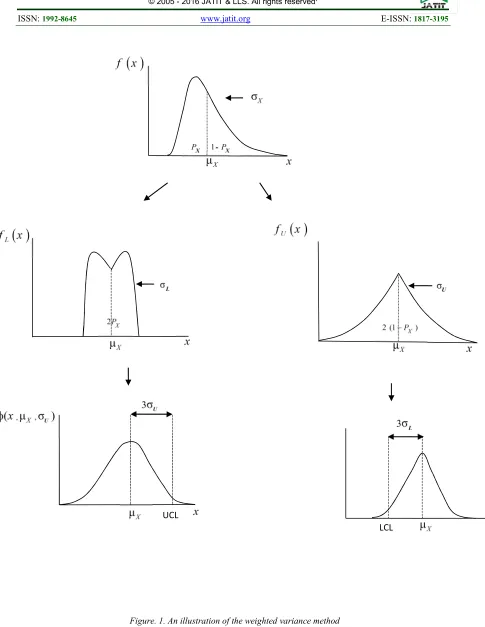
According to Choobineh and Ballard [7], the basic idea of the weighted variance (WV) method is that a skewed distribution can be split into two segments at its mean, where each segment is used to create a new symmetric distribution. The two new distributions created from the original skewed distribution have the same mean but different standard deviations. The WV method uses the two created symmetric distributions to set up the limits of the WV control chart. Specifically, one of the two new distributions is used to compute the upper control limit, while the other is used to compute the lower control limit of the WV control chart. Since the WV method uses a multiple of the standard deviation to establish the control limits, it requires determination of the standard deviations of the two new symmetrical distributions. Choobineh and Ballard [7] developed a method to approximate the variance of the two distributions. This method of approximating the variance is summarized as follows:

Let φ ⋅( ) and Φ ⋅( ) denote the standard normal, N(0,1), pdf and cdf, respectively. Let f x

( )

in Figure 1 be the probability density function (pdf) of quality characteristic

X

, from a skewed distribution;

X

µ and σX be the mean and standard deviation

of X respectively, and PX =P X

(

≤ µX

)

. The

weighted variance method was initially proposed by Choobineh and Ballard [7]. This method is based on the idea that the probability density function f x

( )

can be split into two new symmetrical functions, fL

( )

x and fU

( )

x

having the same mean µX but different

variances, 2

L

σ for fL

( )

x and

2

U

σ for fU

( )

x

(see Figure 1). fL

( )

x and fU

( )

x are replaced

by two normal distributions

(

_, _,

)

(

)

1

X L X L L

x  x − 

φ µ σ = φ_ − µ σ _ σ and

(

_, _,

)

(

)

1

X U X U U

x  x − 

φ µ σ = φ_ − µ σ _ σ , having the

same mean

µ

X and variances

2

L

σ and 2

U

σ , respectively (see Figure 1). This differs from the standard S control chart in that the standard deviation is multiplied by two different factors. One factor is used for the upper control limit (UCL), while the other is used for the lower control limit (LCL). Assume that,

(

X

)

X

P

X

P

=

≤

µ

, is the probability that random variable X is less than or equal to its mean

µ

_X. Then the UCL factor is 2PX and

the LCL factor is 2 1

(

−P_X

)

(for more details see Choobineh and Ballard [7]). See Figure 1 for an illustration of the weighted variance method.

The WV-S control chart suggested by Khoo et al. [11] is set up by plotting the sample standard deviations,

S

i for i =1, 2, …, based on the

following limits in Khoo et al. [11]:

UCLWV−S =µS+3σS 2PX

(6) and

LCL_WV₋_S =µ_S −3σ_S 2 1

(

−P_X

)

, (7)

where µS and σs are the mean and standard

deviation of S, respectively. Note that when 1

2

X

P = the WV-S control chart reduces to the standard S control chart. If the process parameters are unknown, the limits of the WV-S are:

( )

2

4 WV

4

3 1

ˆ

UCL S 1 2 X U

C

S P B S

C −  ₋ _′    = + =  ′    (8) and

( )

(

)

2 4 WV 4 3 1 ˆ

LCL S 1 2 1 X L

C

S P B S

(4)

64 Here, 4

( )

X

E S C

σ

′ = is a constant for a given

skewed population and 1

r i i S S r =

=

∑

is the average

of the sample standard deviations estimated from r preliminary subgroups, while values of BU and

L

B are computed via simulation using SAS 9.3 and

(

)

n

m

X

I

P

m i n j ij X

_×

−

=

∑∑

=1 =1

ˆ

_,

(10)

where m and n are the number of samples in the preliminary data set and the sample size, respectively, and I(x) = 1 if x ≥ 0 or I(x) = 0, otherwise.

2.2.2 A scaled weighted variance (SWV) method

Castagliola [3] suggested a new approach, called the scaled weighted variance method to improve the performance of the weighted variance method. The functions fL

( )

x and fU

( )

x are

not simply replaced by two normal probability density distributions φ

(

x,

µ σ

_X, _L

)

and

(

x,

µ σ

X, U

)

φ , but are replaced by two

“bell-shaped” functions φ

(

x,

µ σ

_X, _L, 2P_X

)

and

(

)

(

x,µ σ_X, _U, 2 1 P_X

)

φ − centered on

µ

_X, having 2

L

σ and 2

U

σ for second central moments and

2PX and 2 1

(

−PX

)

for areas. Castagliola [3]

defined the function φ

(

x,

µ

X, ,t k

)

as

(

)

(

)

3 2

, X, , X .

x k

k

x t k

t t

µ

µ ϕ − 

φ = _ _

 

This function has the following required properties (see Castagliola [3]) for more details about the derivations:

(

x,

µ

X, ,t k dx

)

k +∞

−∞

φ =

∫

(11)

(

x

µ

_X

) (

2 x,

µ

_X, ,t k dx

)

t2. +∞

−∞

− φ =

∫

(12)

Using φ

(

x,

µ

_X, ,t k

)

instead of the probability density function φ

(

x,

µ

X,t

)

gives new limits for

the weighted variance S control chart proposed by Khoo et al. [11].

Proposed scaled weighted variance S control chart (SWV-S) limits:

(

) (

)

1 SWV

UCL 1

4 1 1

X

S S S

X X

P

P P

α

µ − σ

−

 

= + Φ _ − _

− −   (13) and

(

)

1 SWV 1

LCL 1 .

4

X

S S S

X X

P

P P

α

µ − σ

−

 

= − Φ  − 

  (9)

Here,

µ

_S and

σ

_S are the mean and standard deviation of the S respectively, and

α

is Type I error rate (False alarm). Note that, we called this control chart a Scaled Weighted Variance S control chart or SWV-S control chart in short, because the functionφ

(

x,

µ

X, ,t k

)

is scaled by a

factor 3

2 k

t (see Castagliola [3] for more details).

Note also that when 1 2

X

(5)

ISSN: 1992-8645 www.jatit.org E-ISSN: 1817-3195 65

(

)

( )

(

)

2 4 1 SWV 4 ˆ 1

UCL 1 1

ˆ ˆ

4 1 1

X S X X C _P S C P P α − −    ₋ _′     

= _ + Φ _ − _ _

′ − −    _ _    (10) and

( )

2

(

)

4 1 SWV 4 ˆ 1 1

LCL 1 1

ˆ ˆ 4 X S X X P C S C P P α + − −  ₋ _′ ₋     

= _ − Φ _ − _ _ ′       (11)

Here, 4

( )

X

E S C

σ

′ = is a constant for a given

skewed population and 1

r i i S S r =

=

∑

is the average

of the sample standard deviations estimated from r preliminary subgroups.

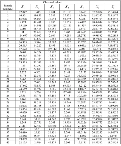
3. AN ILLUSTRATIVE EXAMPLE

The data in table 1 are generated from a Weibull distribution for the purpose of illustration, the data consist of 200 skewed observations grouped into 40 subgroups of size n = 5 each. These data are supposed to correspond to an in-control process. The shape parameter,β , is chosen to be 0.9987 so that the skewness, α₃ is 2, and scale parameter,

λ

is chosen to be 30.50. From these data, we obtained ˆµ = 31.17,

σ

ˆ = 32.43 and C₄′ = 0.8688. We also observe from the data that 125 observations fall below ˆµ. Thus, Pˆ_X = 0.625 from Equation (5). By assuming

0.0027

α

= , the SWV-S chart’s control limits computed using Equations (10) and (11) are equal to UCL_SWV−_S= 88.527 and LCLSWV−S

=-9.978. These limits are compared with those obtained for the WV-S control chart, (UCL_WV−_S

= 82.035 and LCL_WV−_S = -13.545), and the

standard S control chart (UCL_SH−_S =76.349 and

SH S

LCL − = -19.999).From this example, we note

that, the upper control limits obtained for the

SWV-S control chart is further away from the center line than the upper control limits obtained with other methods, and the lower control limit is closer to the center line than the lower limits obtained with the other methods. From Figure 2, we observe that all points fall within control limits of the SWV-S chart, indicating that the process is in-control. On the other hand, two points are on the board of UCL_SH−_s of the

standard S control, and these two points are plotted close to the UCL_SWV−_S of the WV-S

chart. We note that, the SWV-S control chart performs better than the WV-S and standard S control charts.

4. DISCUSSION

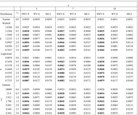
The false alarm rates of the SWV–S chart for many degree of skewness are lower than that of the normal theory value, (see Table 2).Table 3 shows that the probability of detection rates of the SWV–S chart for skewed populations are reasonably close to that of the exact –S chart for skewed distribution .These results show the robustness of the SWV–S chart to violations of the normality assumption. These results, combined with the fact that the SWV–S chart outperforms of the Shewhart S and WV-S control charts for skewed populations in detecting small, moderate and large shifts in the process standard deviation (see Tables 3) make the SWV–S chart appealing to practitioners. The chart with the lowest false alarm and the highest probability of out-of-control detections for most level of skewness and sample size, n is assumed to be have a better performance. Hence, our proposed SWV-S chart have this properties. However, the practitioners have confidence to choose this chart as a good alternative to the Shewhart S and WV-S control charts for monitoring process dispersion when the distributions are skewed.

5. PERFORMANCE EVALUATION OF

THE PROPOSED SWV-S _CONTROL

(6)

66 The SWV−S control chart is compared with the WV-S control chart for skewed data proposed by Khoo et al. [11] and standard S control chart, in terms of the false alarm rate. In terms of the Probabilities of out-of-control detections, the proposed SWV-S control chart is compared with the exact method, WV-S and standard S control charts. A Monte Carlo simulation is conducted using SAS 9.3 to compute the false alarm rates and Probabilities of out-of-control detections. The false alarm rate of a control chart is defined as the proportion of subgroup points plotting beyond the limits of the chart, given that the process is actually in-control. On the contrary, the probability of out-of-control detection measures the ability of a chart in responding to a shift in the process and it represents the proportion of subgroup points plotting beyond the limits of the chart when the process has shifted. All the charts considered in this paper are designed based on an in-control ARL of 370. A shift in the process standard deviation is represented by σ₁=δ σ_X , where

δ

∈

{1.1, 1.3, 1.5, 2.0, 2.5, 3.0, 3.5, 4.0} is the magnitude of a shift, in process standard deviation. The skewed distributions considered here, are Weibull, lognormal and gamma because they represent a wide variety of shapes from symmetric to highly skewed. For the sake of comparison, the standard normal distribution is also considered. For convenience, a scale parameter of one is used for the Weibull and gamma distributions, while a location parameter of zero is selected for the lognormal distribution since the skewness does not depend on the parameters of these distributions. Note that

P

_X for the Weibull, lognormal and gamma distributions are :

PX 1 exp

(

1 1

)

β

 _ _ 

= − _− Γ +_ _ _

 

  (14)

( )

2

X

P = Φ

ω

(15) and

PX =F

( )

γ (16)

respectively, where β,

ω

and γ are the shape parameters (see Khoo et al., [10] and Khoo et al., [11]):. Here,

Γ ⋅

( )

is the gamma function, while

( )

Φ ⋅

and

F

( )

⋅

are the lognormal and gamma distribution functions, respectively. In the case of the false alarm rates, the skewness coefficients considered are

α

₃

∈

{0.5, 1.0, 1.5, 2.0, 2.5, 3.0}, while skewness coefficient,

α

₃=2 is considered in the case of the probability of out-of-control detection. The sample sizes, n

∈

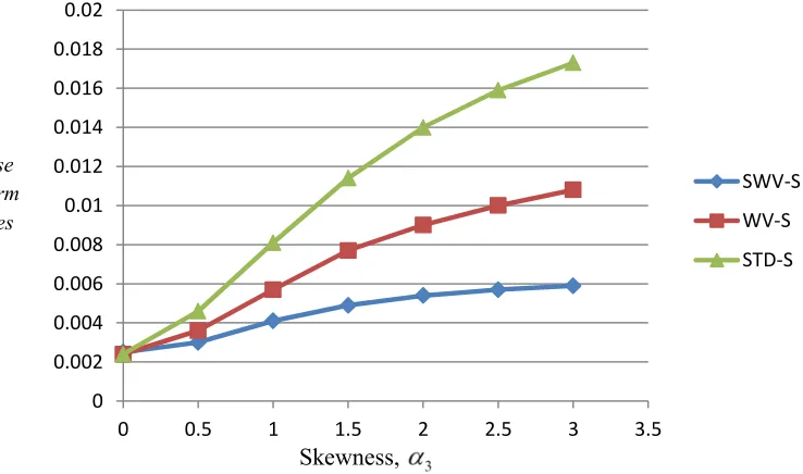
{5, 7, 10} are considered for the false alarm rate and the probability of out-of-control detection. The false alarm rate and probability of out-of-control detection are obtained based on 10000 simulation trials. The simulated results are tabulated in Table 2 and 3 for the false alarm rate and probability of out-of-control detection, respectively. Table 2 shows that the proposed SWV-S control chart has lower false alarm rate than the WV-S control chart for almost all levels of skewnesses and sample sizes, when the distributions are Weibull, lognormal and gamma. Table 3 shows that the probabilities of out-of-control detections of the proposed SWV-S charts are closer to those of the exact S chart than those of the WV-S and standard S control charts. Figures 3 to 5 presented the false alarm rate when sample sizes, n 5, 7 and 10 for the Weibull, lognormal and gamma distributions respectively, the figures show that the false alarm rate of the proposed SWV-S control chart is lower than all the charts considered in this paper for all levels of skewnesses and sample sizes. In general, the proposed SWV-S control chart provides good performances in term of false alarm rate and probability of out-of-control detection for all levels of skewnesses, sample sizes and magnitudes of shifts.

6. CONCLUSIONS

[image:6.612.90.282.553.664.2]

(7)

67 SWV-S control chart offers considerable improvement over the WV-S and standard S control charts when it is desirable for the false alarm rate to be closed to the conventional 0.0027. In the case of the probability of out-of-control detections, the simulation results show that the said probabilities of the proposed SWV-S control chart are closer to the chart constructed by exact S chart than the WV-S and standard S control charts. The findings are based on the SWV-S method instead of relying on the WV-S. Hence, the SWV-S chart can act as a favorable substitute to the existing WV-S and standard S control charts in the evaluation of the speed of a chart to detect shifts in process dispersion, when the underlying distribution is skewed. In conclusion, this study would help practitioners in deciding which type of chart to be used in process of monitoring as part of quality control procedures. Another focus for future research can deal with the construction of scaled weighted variance (SWV) method with EWMA and CUSUM control charts for skewed populations. Incorporating the scaled weighted variance (SWV) method to construct synthetic S chart for skewed populations is another potential topic for further research.

REFERENCES:

[1] Atta AMA, Shoraim MHA and Yahaya SSS. A Multivariate EWMA Control Chart for Skewed Populations using Weighted Variance Method. Int. Res. J. of Sci. & Engg., 2014; 2 (6):191-202.

[2] Bai, D. S. and Choi, I. S. (1995).

X

and R control charts for skewed populations. Journal of Quality Technology, 27, 120 – 131.

[3] Castagliola, P. (2000).

X

control chart for skewed populations using a scaled weighted variance method. International Journal of Reliability, Quality and Safety Engineering, 7, 237 – 252.

[4] Chan, L. K. and Cui, H. J. (2003). Skewness correction

X

and R charts for skewed distributions. Naval Research Logistics, 50, 555 – 573.

[5] Chang, Y. S. and Bai, D. S. (2001). Control charts for positively-skewed populations with weighted standard deviations. Quality and Reliability Engineering International, 17, 397 –406.

[6] Chen, Y. K. (2004). Economic design of

X

control charts for non-normal data using variable sampling policy. International Journal of Production Economics, 92, 61-74.

[7] Choobineh, F. and Ballard, J.L. (1987). Control-limits of QC charts for skewed distribution using weighted variance. IEEE Transactions on Reliability, 36, 473–477. [8] Dou, Y. and Sa, P. (2002). One-sided control

charts for the mean of positively skewed distributions. Total Quality Management, 13, 1021 – 1033.

[9] Khoo, M. B. C., Atta, A. M. A and Wu, Z. (2009b). A Multivariate Synthetic Control Chart for Monitoring the Process Mean Vector of Skewed Populations Using Weighted Standard Deviations. Communications in Statistics – Simulation

and Computation,38, 1493 – 1518.

[10] Khoo, M. B. C., Wu, Z. and Atta, A. M. A. (2008). A Synthetic Control Chart for Monitoring the Process Mean of Skewed Populations based on the Weighted Variance Method. International Journal of

Reliability, Quality and Safety

Engineering,15, 217 – 245.

[11] Khoo, M. B.C., Atta, A.M. A. and Chen, C-H.. (2009a). Proposed

X

and S control charts for skewed distributions, Proceedings of the International Conference on Industrial Engineering and Engineering Management (IEEM 2009), Dec. pp. 389-393, Hong Kong.

[12] Teh, S. Y., Khoo, M. B. C., Ong, K. H., and Teoh, W. L., Comparing the Median Run Length (MRL) Performances of the Max-EWMA and Max-DMax-EWMA Control Charts for Skewed Distributions Proceedings of the 2014 International Conference on Industrial Engineering and Operations

Management Bali, Indonesia, January 7 –

9, 2014.

[13] Montgomery, D.C. (2009). Introduction to Statistical Quality Control. (6thedition). John Wiley & Sons, Inc., New York. [14] Nichols, M. D. and Padgett, W. J. (2005). A

(8)

68 [15] Tsai, T. R. (2007). Skew normal distribution

and the design of control charts for averages. International Journal of

Reliability, Quality and Safety

Engineering, 14, 49 – 63.

[16] Wu, Z. (1996). Asymmetric control limits of the chart for skewed process distributions. International Journal of

Quality and Reliability Management, 13,

49 – 60.

[17] Yourstone, S. A. and Zimmer, W. J. (1992). Non-normality and the design of control charts for averages. Decision Sciences, 23, 1099 – 1113

.

(9)

69

UCL

[image:9.612.73.558.63.690.2]

LCL

(10)

[image:10.612.117.486.483.701.2]

70

Figure2. S type control charts for the SWV, WV and standard S methods using simulated data from a skewed distribution

Figure 3. False alarm rates for SWV-S, WV-S and STD-S control charts for sample size, n=5 and various skewnesses, Weibull Distribution

0 0.002 0.004 0.006 0.008 0.01 0.012 0.014 0.016 0.018 0.02

0 0.5 1 1.5 2 2.5 3 3.5

SWV-S

WV-S

STD-S

Skewness,

False Alarm Rates

-40 -20 0 20 40 60 80 100

1 3 5 7 9 11 13 15 17 19 21 23 25 27 29 31 33 35 37 39

(11)

71

Figure 4. False alarm rates for SWV-S, WV-S and STD-S control charts for sample size, n=7 and various skewnesses, Lognormal Distribution

Figure 5. False alarm rates for SWV-S, WV-S and STD-S control charts for sample size, n=10 and various skewnesses, gamma distribution.

0 0.002 0.004 0.006 0.008 0.01 0.012 0.014 0.016 0.018 0.02

0 0.5 1 1.5 2 2.5 3 3.5

SWV-S

WV-S

STD-S

0 0.002 0.004 0.006 0.008 0.01 0.012 0.014 0.016

0 0.5 1 1.5 2 2.5 3 3.5

SWV-S

WV-S

STD-S

Skewness,

False Alarm Rates

(12)

[image:12.612.115.529.114.613.2]

72

Table 1: An example of illustration using simulated data from a skewed population (Weibull distribution)

Observed values Sample

number, i

X

1

X

2

X

3

X

4

X

5

X

i

S

i

(13)

[image:13.612.84.536.111.488.2]

73

Table. 2: False Alarm rates of the SWV-S, WV-S and standard –S control charts

n

5 7 10

Distribution α3 _SWV-S _WV-S _SH-_S _SWV-S _WV-S _SH-_S _SWV-S _WV-S _SH-_S

Normal 0.0 0.0039 0.0039 0.0039 0.0035 0.0035 0.0035 0.0031 0.0031 0.0031

Weibull

β

3.6286 0.0 0.0025 0.0024 0.0024 0.0023 0.0023 0.0022 0.0023 0.0023 0.0022

2.2266 0.5 0.0030 0.0036 0.0046 0.0027 0.0032 0.0040 0.0025 0.0029 0.0035 1.5688 1.0 0.0041 0.0057 0.0081 0.0034 0.0049 0.0072 0.0030 0.0043 0.0063 1.2123 1.5 0.0049 0.0077 0.0114 0.0041 0.0067 0.0102 0.0036 0.0057 0.0090 0.9987 2.0 0.0054 0.0090 0.0140 0.0046 0.0080 0.0127 0.0040 0.0070 0.0114 0.8598 2.5 0.0057 0.0100 0.0159 0.0049 0.0091 0.0147 0.0044 0.0081 0.0134 0.7637 3.0 0.0059 0.0108 0.0173 0.0052 0.0099 0.0162 0.0046 0.0090 0.0151 Lognormal

ω

0.0010 0.0 0.0061 0.0061 0.0061 0.0014 0.0014 0.0014 0.0088 0.0088 0.0088

0.1656 0.5 0.0046 0.0054 0.0065 0.0043 0.0050 0.0060 0.0038 0.0045 0.0053 0.3170 1.0 0.0066 0.0084 0.0107 0.0062 0.0078 0.0100 0.0056 0.0072 0.0092 0.4484 1.5 0.0079 0.0105 0.0138 0.0074 0.0099 0.0139 0.0068 0.0092 0.0124 0.5593 2.0 0.0084 0.0117 0.0158 0.0080 0.0111 0.0152 0.0075 0.0105 0.0144 0.6525 2.5 0.0087 0.0124 0.0169 0.0083 0.0118 0.0165 0.0078 0.0113 0.0157 0.7315 3.0 0.0087 0.0127 0.0176 0.0083 0.0122 0.0172 0.0079 0.0117 0.0166 Gamma

γ

38000 0.0 0.0039 0.0039 0.0040 0.0033 0.0033 0.0033 0.0028 0.0028 0.0028

(14)

[image:14.612.52.566.122.456.2]

74

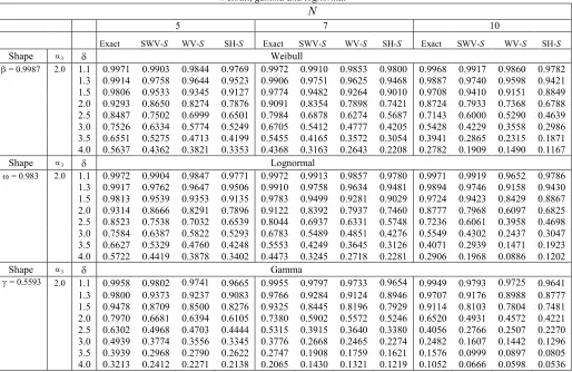
Table 3: Probabilities of out-of-control detections for the various charts when the underlying distributions are Weibull, gamma and lognormal

N

5 7 10

Exact SWV-S WV-S SH-S Exact SWV-S WV-S SH-S Exact SWV-S WV-S SH-S

Shape α3 δ Weibull

β = 0.9987 2.0 1.1 0.9971 0.9903 0.9844 0.9769 0.9972 0.9910 0.9853 0.9800 0.9968 0.9917 0.9860 0.9782 1.3 0.9914 0.9758 0.9644 0.9523 0.9906 0.9751 0.9625 0.9468 0.9887 0.9740 0.9598 0.9421 1.5 0.9806 0.9533 0.9345 0.9127 0.9774 0.9482 0.9264 0.9010 0.9708 0.9410 0.9151 0.8849 2.0 0.9293 0.8650 0.8274 0.7876 0.9091 0.8354 0.7898 0.7421 0.8724 0.7933 0.7368 0.6788 2.5 0.8487 0.7502 0.6999 0.6501 0.7984 0.6878 0.6274 0.5687 0.7143 0.6000 0.5290 0.4639 3.0 0.7526 0.6334 0.5774 0.5249 0.6705 0.5412 0.4777 0.4205 0.5428 0.4229 0.3558 0.2986 3.5 0.6551 0.5275 0.4713 0.4199 0.5455 0.4165 0.3572 0.3054 0.3941 0.2865 0.2315 0.1871 4.0 0.5637 0.4362 0.3821 0.3353 0.4368 0.3163 0.2643 0.2208 0.2782 0.1909 0.1490 0.1167 Shape α3 δ Lognormal

ω = 0.983 2.0 1.1 0.9972 0.9904 0.9847 0.9771 0.9972 0.9913 0.9857 0.9780 0.9971 0.9919 0.9652 0.9786 1.3 0.9917 0.9762 0.9647 0.9506 0.9910 0.9758 0.9634 0.9481 0.9894 0.9746 0.9158 0.9430 1.5 0.9813 0.9539 0.9353 0.9135 0.9783 0.9499 0.9281 0.9029 0.9724 0.9423 0.8429 0.8867 2.0 0.9314 0.8666 0.8291 0.7896 0.9122 0.8392 0.7937 0.7460 0.8777 0.7968 0.6097 0.6825 2.5 0.8523 0.7538 0.7032 0.6539 0.8044 0.6937 0.6331 0.5748 0.7236 0.6061 0.3958 0.4698 3.0 0.7584 0.6387 0.5822 0.5293 0.6783 0.5489 0.4851 0.4276 0.5549 0.4302 0.2437 0.3047 3.5 0.6627 0.5329 0.4760 0.4248 0.5553 0.4249 0.3645 0.3126 0.4071 0.2939 0.1471 0.1923 4.0 0.5722 0.4419 0.3878 0.3402 0.4473 0.3245 0.2718 0.2281 0.2906 0.1968 0.0886 0.1202 Shape α3 δ Gamma