Modelling dependency structural of the wind energy in Lebanon

Full Length Research Article

MODELLING DEPENDENCY STRUCTURAL OF THE WIND ENERGY IN LEBANON

Hussein Khraibani and *Zaher Khraibani

Lebanese University, Faculty of Sciences, Department of Applied Mathematics, Hadat, Lebanon

ARTICLE INFO ABSTRACT

For several decades, wind power is experiencing tremendous growth, however, the production of wind energy depends on wind intensity, strongly volatile, and is therefore characterized by a high degree of uncertainty. Planning the installation of a wind farm for several stations requires the assessment of the risk which in turn results in an assessment of the variability in production. Longevity, it starts with the recognition of the links between the various stations. The objective of this article is to develop a dependency structure assessment approach between different stations in Lebanon. The database used includes daily subsistence wind speeds of fourteen stations in Lebanon over a period of 6 years, from October 28th, 2009 until March 15th, 2016 and freely available on the NOAA network of American government. This database are used to estimate the necessary models such as, the univariate time series which will be modeled by the ARIMA process. We will establish a structure of spatial dependence of the innovations of these processes between different stations by using the copulas theory.

Copyright©2017, Hussein Khraibani and Zaher Khraibani.This is an open access article distributed under the Creative Commons Attribution License, which permits unrestricted use, distribution, and reproduction in any medium, provided the original work is properly cited.

INTRODUCTION

The wind is a source of energy that is continually renewed by natural phenomena. Wind energy is growing in different countries of the world, growing at 30% per year. This development of the wind energy is due to the environmental qualities of this form of energy but also to other economic factors such as; speed of installation, cost predictability over the long term, energy independence, financial aid, etc. At the end of 2033, wind power represents 218,500 megawatts (MW) of installed capacity in the worldwide with a significant growth (+ 21% capacity in 2011) ( Nicola Armaroli, 2011). The experts from the World Wind Energy Council predict that wind energy will continue to grow globally, particularly in emerging countries such as Brazil, India and Mexico (Fthenakis, 2009). This energy began in Egypt in the 1990s with the wind farms in Zaafarana generating 225 MW. More recently, Egypt has tendered for the construction of a 200 MW wind farm in the Gulf of El-Zayt. In Jordan, the central power generation company has set up two pilot wind farm projects: a 320 KW fleet in Ibrahimia, installed in 1988, and a 1.2 MW fleet in Hofa. In Syria, studies on wind speed have been carried out, but so far there is no large wind farm (Allen et al. 2008). In the literature there exists various studies on the wind energy such as the spatial dependence of the wind (Oliver Grothe et al., May 2011), and the distribution of the optimal wind energy, based on the copula, in the authors modeled the marginal distribution and structure of the wind speed dependence of the regions considered, which is the first to systematically analyze wind farm networks of different sizes.

Moreover there exist a new method for generating the Wind Speed Time Series (WSTS) dependency based on copula theory and univariate time series. An Autoregressive Moving Average (ARMA) model and multivariate GARCH model are applied to represent the time series of wind speed. Through the review of literature, this article will be structured as follows. In a first part, we will see how modelling the wind speed for each associated station. Generally, univariate time series will be modeled by ARMA-GARCH type processes. Then we will choose the one that best adapts model to create a possible link between several stations. In addition we identify stations (sites) and extract the daily wind speed data for each station over a given period (from October 2009 to March 2016). After seasonal adjustment, we estimate a stationary stochastic process. The innovations of each estimated stochastic process will establish the temporal and spatial dependence between the studied stations by using the copulas theory.

*Corresponding author: Zaher Khraibani,

Lebanese University, Faculty of Sciences, Department of Applied Mathematics, Hadat, Lebanon.

ISSN: 2230-9926

International Journal of Development Research

Vol. 07, Issue, 01, pp.11255-11266, January,2017

International Journal of

DEVELOPMENT RESEARCH

Article History:

Received 17th _{October, 2016}

Received in revised form 27th _{November, 2016}

Accepted 04th _{December, 2016}

Published online 30th _{January, 2017}

Key Words:

MATERIALS AND METHODS

Wind Energy in the World

We give in this subsection some descriptive analysis of the distribution of the wind energy in the world.

The importance of wind energy in Lebanon comes to solve the problem of the electricity sector for several years. Today, the electricity sector faces two major problems, one of a technical

view, there is a large gap between national demands, which needs 2,400MWand supply, which is 1,500MW. Moreover, these numbers do not take into account the energy needs of the millions of

war in Syria. The production is mainly using during the peak periods (Harajli et al., 2011). case it is also a response to electricity production.

Figure 1. The first 10 countries new capacity installed betweenJanuary

Ideally, Lebanon could achieve a 50% ratio of renew

wind power. Certainly it would not be obvious to put wind turbines everywhere but, unlike solar energy, the wind turbine produces more power over a restricted space. If photovoltaic

the land around the wind turbine can be exploited. In Lebanon, it is a response to local pollution, which is felt between 10 15km around the power stations that produce fuel oil

is generally cheaper than solar, depending on the project, the difference may vary from 30% to 100%, even though this differe is now tending to fade. Finally, it is a sustainable

independence. In 2009, at the Copenhagen summit, Lebanon had committeditself to produce 12% of its energy from renewable sources by 2020 (Al Zohbi et al., 2041). It is therefore ur

source.

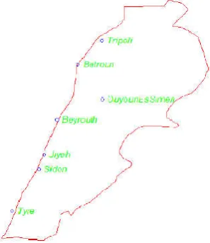
Figure 2. Geographical location of station on Lebanese territory

Databases of the wind energy in Lebanon

The acquisition of historical databases allows one to observe

these long-term wind variations, a. The using system for the measure of wind speed is the GFS (Global Forecast System). It is calculated by the National Centers for Environmental Predict

Atmospheric Administration), NWS (National Weather Service), USA.

with a frequency of 8 observations per day (one measurement every 3 hours) and then

to obtain the daily wind speed in 7 stations (Figure 2), (Jiyeh, Sidon, Tyre in south of Lebanon, Beirut the Capital, Batroun Tripoli in north of Lebanon and Ouyoun Es Simen in Mount Lebanon).

11256 Hussein Khraibani and Zaher Khraibani, Modelling

analysis of the distribution of the wind energy in the world.

The importance of wind energy in Lebanon comes to solve the problem of the electricity sector for several years. Today, the electricity sector faces two major problems, one of a technical nature and the other of a financial nature.

view, there is a large gap between national demands, which needs 2,400MWand supply, which is 1,500MW. Moreover, these numbers do not take into account the energy needs of the millions of Syrian refugees who were installed in Lebanon during the war in Syria. The production is mainly using the fossil fuels and the demand exceeds the supply and the breakdowns are frequent 2011). In general, renewable energies are a response to global warming, in the Lebanese case it is also a response to electricity production.

Figure 1. The first 10 countries new capacity installed betweenJanuary - December 2015

Ideally, Lebanon could achieve a 50% ratio of renewable energy in 20 years, and some of this production could be provided by wind power. Certainly it would not be obvious to put wind turbines everywhere but, unlike solar energy, the wind turbine produces more power over a restricted space. If photovoltaic panels are installed in an agricultural area, agriculture is killed, while the land around the wind turbine can be exploited. In Lebanon, it is a response to local pollution, which is felt between 10 15km around the power stations that produce fuel oil. With wind power, the purchase price for the consumer is much lower. Wind is generally cheaper than solar, depending on the project, the difference may vary from 30% to 100%, even though this differe is now tending to fade. Finally, it is a sustainable production that consumes only wind and contributes to the country's energy independence. In 2009, at the Copenhagen summit, Lebanon had committeditself to produce 12% of its energy from renewable 2041). It is therefore urgent for Lebanon to find a solution to cover demand with a clean energy

Figure 2. Geographical location of station on Lebanese territory

The acquisition of historical databases allows one to observe first a trend of change of the wind regime over the long term. The using system for the measure of wind speed is the GFS (Global Forecast System). It is calculated by the National Centers for Environmental Prediction (NCEP) a department of NOAA (National Oceanic and Atmospheric Administration), NWS (National Weather Service), USA. The data are obtained by measurements of wind speed with a frequency of 8 observations per day (one measurement every 3 hours) and then we calculated the average of the wind speed to obtain the daily wind speed in 7 stations (Figure 2), (Jiyeh, Sidon, Tyre in south of Lebanon, Beirut the Capital, Batroun Tripoli in north of Lebanon and Ouyoun Es Simen in Mount Lebanon).

Zaher Khraibani, Modelling dependency structural of the wind energy in Lebanon

analysis of the distribution of the wind energy in the world.

The importance of wind energy in Lebanon comes to solve the problem of the electricity sector for several years. Today, the nature and the other of a financial nature. From a technical point of view, there is a large gap between national demands, which needs 2,400MWand supply, which is 1,500MW. Moreover, these Syrian refugees who were installed in Lebanon during the the fossil fuels and the demand exceeds the supply and the breakdowns are frequent energies are a response to global warming, in the Lebanese

December 2015

able energy in 20 years, and some of this production could be provided by wind power. Certainly it would not be obvious to put wind turbines everywhere but, unlike solar energy, the wind turbine panels are installed in an agricultural area, agriculture is killed, while the land around the wind turbine can be exploited. In Lebanon, it is a response to local pollution, which is felt between 10 and . With wind power, the purchase price for the consumer is much lower. Wind is generally cheaper than solar, depending on the project, the difference may vary from 30% to 100%, even though this difference production that consumes only wind and contributes to the country's energy independence. In 2009, at the Copenhagen summit, Lebanon had committeditself to produce 12% of its energy from renewable gent for Lebanon to find a solution to cover demand with a clean energy

first a trend of change of the wind regime over the long term. Unlike The using system for the measure of wind speed is the GFS (Global Forecast System). It is ion (NCEP) a department of NOAA (National Oceanic and The data are obtained by measurements of wind speed we calculated the average of the wind speed to obtain the daily wind speed in 7 stations (Figure 2), (Jiyeh, Sidon, Tyre in south of Lebanon, Beirut the Capital, Batroun and

Stochastic model

In this subsection, we will adjust a time series model to th

series univariate with seasonal (ARMA) for modelling the wind speed data. The most time series have a tendency and / or a seasonal oscillation (on shorter time scales than the year) characterizes the wind in a Station, so it is more predictable. The wind regime will not be the same in winter as in summer.

in 14 stations in different regions in Lebanon from 28/11/2009 to 15/3/2016.

We consider a time series succession of observations over time

The stationarity has an important role in the prediction of time series which possess th

( ) = ; ( ) = = ; (

If the series is stationary without differentiation then it is modeled by an ARMA(p, q)

successive differentiations to yield the series stationary and the initial series will be modeled by an ARIMA(p, d, q) proces d is the number of differentiations necessary to obtain a stationary series (Phillips, 19

stationarity among these tests: Kwiatkowski "adf" (Dickey & Fuller, 1979), and the Phillips

namely the augmented Dickey-Fuller test which the hypotheses test

stationary. In order, the sites chosen for the article are: Jiyeh (dsj), Sidon (dssid) a

Capital, Batroun (dsba) and Tripoli (dstr) in the North and Ouyoun Es Simen Dsouy) at Mount Lebanon. However, the wind speed distributions of these sites are asymmetric and have seasonal effects, so they have t

Modeling and interpretation of results

This transformation allows the obtaining of symmetric values using the Box Cox and Tukey (Box

the proper transformations of this series are carried out, one returns to a constant tendency in time and to a nonvolatile se Box-Cox transformation is given by the transformation formula:

( ) =

− 1

≠ 0

= 0

With is a parameter estimated by the maximum likelihood method takes the values between [ describes re-expressing variables using a power transformation:

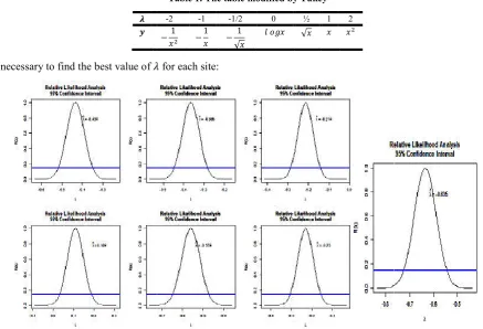
First it is necessary to find the best value of

Figure 3. Curve of the best value of

The transformation of each site:

subsection, we will adjust a time series model to the wind speed data for each site (Benth

series univariate with seasonal (ARMA) for modelling the wind speed data. The most time series have a tendency and / or a oscillation (on shorter time scales than the year) characterizes the wind in a Station, so it is more predictable. The wind regime will not be the same in winter as in summer. The selection of the station is important and the wind speed data is distributed in 14 stations in different regions in Lebanon from 28/11/2009 to 15/3/2016.

We consider a time series succession of observations over time{ , = 1,2, … , }, ∈ .

The stationarity has an important role in the prediction of time series which possess the following conditions:

( , ) = .

If the series is stationary without differentiation then it is modeled by an ARMA(p, q) process. Otherwise, we perform a successive differentiations to yield the series stationary and the initial series will be modeled by an ARIMA(p, d, q) proces

d is the number of differentiations necessary to obtain a stationary series (Phillips, 1988) There exist a several tests to detect the stationarity among these tests: Kwiatkowski-Phillips-Schmidt-Shin "kpss" (Kwiatkowski et al., 1992), augmented Dickey "adf" (Dickey & Fuller, 1979), and the Phillips - Perron "pp". In the rest of this paper, we use the simplest and classical test,

Fuller test which the hypotheses test : The model is non-stationary and

In order, the sites chosen for the article are: Jiyeh (dsj), Sidon (dssid) and Tyre (dsty) in South Lebanon, Beirut (dsb) Capital, Batroun (dsba) and Tripoli (dstr) in the North and Ouyoun Es Simen Dsouy) at Mount Lebanon. However, the wind speed distributions of these sites are asymmetric and have seasonal effects, so they have to be processed and seasonally adjusted.

This transformation allows the obtaining of symmetric values using the Box Cox and Tukey (Box

the proper transformations of this series are carried out, one returns to a constant tendency in time and to a nonvolatile se Cox transformation is given by the transformation formula:

is a parameter estimated by the maximum likelihood method takes the values between [ expressing variables using a power transformation:

Table 1. The table modified by Tukey

-2 -1 -1/2 0 ½ 1 2

−1 −1 − 1

√

√

for each site:

Figure 3. Curve of the best value of for each site

(Benth et al., 2010), proposed the time series univariate with seasonal (ARMA) for modelling the wind speed data. The most time series have a tendency and / or a oscillation (on shorter time scales than the year) characterizes the wind in a Station, so it is more predictable. The wind The selection of the station is important and the wind speed data is distributed

e following conditions:

process. Otherwise, we perform a successive differentiations to yield the series stationary and the initial series will be modeled by an ARIMA(p, d, q) process where 88) There exist a several tests to detect the 1992), augmented Dickey-Fuller aper, we use the simplest and classical test, stationary and : The model is nd Tyre (dsty) in South Lebanon, Beirut (dsb) Capital, Batroun (dsba) and Tripoli (dstr) in the North and Ouyoun Es Simen Dsouy) at Mount Lebanon. However, the wind speed

o be processed and seasonally adjusted.

This transformation allows the obtaining of symmetric values using the Box Cox and Tukey (Box et al., 1964) transformations. If the proper transformations of this series are carried out, one returns to a constant tendency in time and to a nonvolatile seasonality.

According to the application on R library "forecast"

following Table:

Table 2. The best transformation for each site (graphically and by Skweness test)

Station Jiyeh Beirut Batroun Ouyoun Es Siman Sidon

Tripoli Tyre

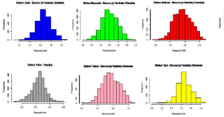
Viewing data after transformations given by the following graphics:

Figure 4. Histogram of each Station after transformation

Based on Figure 4we see that our distributions will be almost symmetrical. Hence the hypothesis of symmetry of the data is satisfied.

Figure 5. Curve of the wind speed of each Station after the transformation 11258 Hussein Khraibani and Zaher Khraibani, Modelling dependency structural of the wind energy in Lebanon

"forecast" we compare the different transformations for each site, so we obtain the

Table 2. The best transformation for each site (graphically and by Skweness test)

Tukey transformation

Best transformation

Skweness -0.434 −1⁄

= − 1 0.01305953

-0.365 −1⁄

= − 1 0.01956873

-0.214 −1⁄

= − 1 0.006445448

Ouyoun Es Siman 0.109 ( )

= 1

√

-0.03040134 -0.559 −1⁄

= − 1 -0.0621482

-0.23 −1⁄

= − 1 0.01768482

-0.635 −1⁄

= − 1 -0.00327468

Viewing data after transformations given by the following graphics:

Figure 4. Histogram of each Station after transformation

Based on Figure 4we see that our distributions will be almost symmetrical. Hence the hypothesis of symmetry of the data is

5. Curve of the wind speed of each Station after the transformation Zaher Khraibani, Modelling dependency structural of the wind energy in Lebanon

transformations for each site, so we obtain the

Table 2. The best transformation for each site (graphically and by Skweness test)

Skweness 0.01305953 0.01956873 0.006445448

0.03040134 0.0621482 0.01768482 0.00327468

Based on Figure 4we see that our distributions will be almost symmetrical. Hence the hypothesis of symmetry of the data is

From Figure 5 it is clear that there exist a seasonal

stationary series. In a second step, we use these series to extract the innovations and then we validate the property "white

these innovations. Once the validation is complete, the data will be ready to be modeled by the copulas. The transformed variable of the wind speed can therefore be expressed in the form of the equation of the following model:

= + Φ + +

With = ; is the historical mean of the variance and calculated using the following nonlinear (periodic) model:

= + cos(2 + 2)

365 +

The model will be applied individually on each series. The obtained residues for each series will be diagnosed by the ARCH test to be sure that there is no sequence of heteroscedasticity.

station are selected from 28/10/2009 to 15/3/2016, corresponding to 7 years of observations.

Table 3. Periodic series model to calculate the seasonal averages

From Figure 5 it is clear that there exist a seasonal effect. We recall that in this article we interested in a first time to obtain a stationary series. In a second step, we use these series to extract the innovations and then we validate the property "white

s complete, the data will be ready to be modeled by the copulas. The transformed variable of the wind speed can therefore be expressed in the form of the equation of the following model:

is the historical mean of the variance and is the residual. For daily data, the seasonal component calculated using the following nonlinear (periodic) model:

cos(2 + 2)

365

will be applied individually on each series. The obtained residues for each series will be diagnosed by the ARCH test to be sure that there is no sequence of heteroscedasticity. In the following applications, the wind speed measurements of each

selected from 28/10/2009 to 15/3/2016, corresponding to 7 years of observations.

Table 3. Periodic series model to calculate the seasonal averages

effect. We recall that in this article we interested in a first time to obtain a stationary series. In a second step, we use these series to extract the innovations and then we validate the property "white noise" of s complete, the data will be ready to be modeled by the copulas. The transformed variable

For daily data, the seasonal component is

Figure 6. Wind speed curve for each station after transformation with the periodic model

Figure 6gives the appearance of periodic models and measured wind speed data after suitable transformations, we note that for the seven sites, the periodic curves are dissimilar. In the follows we give an example for one station (Jiyeh).

Figure

Figure 8. Autocorrelation and partial autocorrelation functions of seasonally adjusted data for Jiyeh

Visually, we observe the non stationarity of the transformation of the data according to PACF. The Dickey-Fuller test confirms this result (p

11260 Hussein Khraibani and Zaher Khraibani, Modelling

Figure 6. Wind speed curve for each station after transformation with the periodic model

6gives the appearance of periodic models and measured wind speed data after suitable transformations, we note that for the seven sites, the periodic curves are dissimilar. In the follows we give an example for one station (Jiyeh).

Times in days

Figure 7. Seasonally adjusted data for Jiyeh station

Figure 8. Autocorrelation and partial autocorrelation functions of seasonally adjusted data for Jiyeh

Visually, we observe the non stationarity of the transformation of the data according to Figure 7 also according to the ACF and Fuller test confirms this result (p-value = 0.6816> 0.05).

Zaher Khraibani, Modelling dependency structural of the wind energy in Lebanon

Figure 6. Wind speed curve for each station after transformation with the periodic model

6gives the appearance of periodic models and measured wind speed data after suitable transformations, we note that for the seven sites, the periodic curves are dissimilar. In the follows we give an example for one station (Jiyeh).

Figure 8. Autocorrelation and partial autocorrelation functions of seasonally adjusted data for Jiyeh station

Figure 7 also according to the ACF and

Table 4. Test of stationarity for the transformed data in Jiyeh station

Lag p-value

We conclude that the seasonally adjusted series is non differentiation.

Table 5. Test of stationarity for the seasonally adjusted data after differentiation in Jiyeh station

Lag p

After differentiation and based on the results of the Dickey <5%, we reject the null hypothesis ofthe non

became stationary.

Jiyeh Station after differentiation

Figure9. Autocorrelation and partial autocorrelation functions of transformed and seasonally adjusted and differentiated data (d = 1) of Jiyeh Station (dsj)

The series (dsj) is therefore stationary, we will search an ARMA(p, q) model. To know the orders of the AR

will use the correlogram of the stationary series (dsj). Indeed, the simple correlogram permit to identify the number of dela the model MA (q), while the partial correlogram allow to identify the number of delay p of the modelAR (p)

3-7 the PACF decreases slowly and exponentially, whereas the examination of the partial correlation shows us that the series ca be modeled by an MA (3).

Table 6. AIC of the ARIMA processes generated from the transformed data in Jiye

Model ARIMA AIC

In Table 6, it appears that the ARIMA (0,1,3) process model is the best adapted model to the data for Jiyeh station according to the AIC criterion. The following Table 8 contains all estimated parameters of the ARIMA

Table 7. Parameters of the model ARIMA(0,1,3) estimated for

Model ARIMA(0,1,3)

The ARIMA (0,1,3) model has the following form with

(1 − ) = + 1 + + + ⋯ +

= + − 0.5423 − 0.321

Thus, it will be necessary to ensure that the residuals of the estimated series are "white noise", that is the average equal the variance is constantnon-auto-correlated. Consequently, the stationarity of the series and the fact tha

noise" constitute the two essential properties.

Table 4. Test of stationarity for the transformed data in Jiyeh station

400 500 600 700 800

value 0.5073 0.5616 0.8942 0.7609 0.6816

that the seasonally adjusted series is non-stationary so it follows an ARIMA model and then we can make a first

Table 5. Test of stationarity for the seasonally adjusted data after differentiation in Jiyeh station

Lag 100 200 300 400 500 p-Value 0.01 0.01 0.01 0.01 0.0342

After differentiation and based on the results of the Dickey-Fuller test applied over several periods of time, we obtain p <5%, we reject the null hypothesis ofthe non-stationary. So the test confirms the absence of a unit root, consequently the series

Jiyeh Station after differentiation Jiyeh Station after differentiation

Autocorrelation and partial autocorrelation functions of transformed and seasonally adjusted and differentiated data (d = 1) of Jiyeh Station (dsj)

The series (dsj) is therefore stationary, we will search an ARMA(p, q) model. To know the orders of the AR

will use the correlogram of the stationary series (dsj). Indeed, the simple correlogram permit to identify the number of dela the model MA (q), while the partial correlogram allow to identify the number of delay p of the modelAR (p)

7 the PACF decreases slowly and exponentially, whereas the examination of the partial correlation shows us that the series ca

Table 6. AIC of the ARIMA processes generated from the transformed data in Jiye

Model ARIMA (0,1,0) (0,1,1) (0,1,2) (0,1,3) -2694.024 -3077.457 -3405.406 -3431.559

(0,1,3) process model is the best adapted model to the data for Jiyeh station according to 8 contains all estimated parameters of the ARIMA (0,1,3) model.

Table 7. Parameters of the model ARIMA(0,1,3) estimated for Jiyeh station

Coefficients

Model ma1 ma2 ma3

ARIMA(0,1,3) -0.5423 -0.3218 -0.1113

model has the following form with the residual:

− 0.113

Thus, it will be necessary to ensure that the residuals of the estimated series are "white noise", that is the average equal correlated. Consequently, the stationarity of the series and the fact tha

noise" constitute the two essential properties.

stationary so it follows an ARIMA model and then we can make a first

Table 5. Test of stationarity for the seasonally adjusted data after differentiation in Jiyeh station

Fuller test applied over several periods of time, we obtain p-values absence of a unit root, consequently the series

Jiyeh Station after differentiation

Autocorrelation and partial autocorrelation functions of transformed and seasonally adjusted and

The series (dsj) is therefore stationary, we will search an ARMA(p, q) model. To know the orders of the ARMA(p, q)model, we will use the correlogram of the stationary series (dsj). Indeed, the simple correlogram permit to identify the number of delay q of the model MA (q), while the partial correlogram allow to identify the number of delay p of the modelAR (p). According to figure 7 the PACF decreases slowly and exponentially, whereas the examination of the partial correlation shows us that the series can

Table 6. AIC of the ARIMA processes generated from the transformed data in Jiyeh station

(0,1,3) process model is the best adapted model to the data for Jiyeh station according to (0,1,3) model.

Jiyeh station

Figure 10. Representation of the residuals of the ARIMA

Figure 10 shows that the series fluctuates around a constant average. The

indicate that there exist a remarkable volatility, so it is necessary to testing the heteroscedasticity of these residues. process is not stationary in variance, it is advisable to use,

process in order to take into account the volatility and the non

Table 8. Heteroscedasti

Lags p

According to the ARCH test applied to several lags, we find that p

"Absence of an ARCH effect", so there exist a heteroscedasticity and it must be modeled from a GARCH

Choice of the GARCH(p,q) model

Table 9. AIC of the GARCH processes generated from the square residue data A

Model c(0,1) c(1,0) AIC -3520.43 -3464.22

Given the profile of autocorrelation and partial autocorrelation functions, we will choose the GARCH representation that best represents the dynamics of volatility. The best model is GARCH (1,1) having the smallest AIC value

Table 10. Parameters of the GARCH (1,1 ) model estimated at residue of the model

Model Value

ℎ( ) = 0.000111 + 0.0534665 ( ) + 0

T

100 Residual ARIMA(0,1,3) 0 Residual GARCH(1,1) 0.2038

The model chosen is validated. We apply the test of suitability on the residuals of the GARCH (1,1)model.

Independence and normality of residues

Test P-value

Result (Threshold 5%)

11262 Hussein Khraibani and Zaher Khraibani, Modelling dependency structural of the wind energy in Lebanon

Time per day

Figure 10. Representation of the residuals of the ARIMA (0,1,3) process for the Jiyeh station

Figure 10 shows that the series fluctuates around a constant average. The residues of the Jiyeh station of the ARIMA(0,1,3)model indicate that there exist a remarkable volatility, so it is necessary to testing the heteroscedasticity of these residues.

process is not stationary in variance, it is advisable to use, rather than an ARIMA process, but rather an ARIMA process in order to take into account the volatility and the non-linearity of the model.

Table 8. Heteroscedasticity test for the Jiyeh station

Lags 200 300 400

p-value 2.326e-11 2.199e-07 9.277e-06

According to the ARCH test applied to several lags, we find that p-value is close to zero. Therefore we reject the null hypothesis "Absence of an ARCH effect", so there exist a heteroscedasticity and it must be modeled from a GARCH

Table 9. AIC of the GARCH processes generated from the square residue data ARIMA (0,1,3) from Jiyeh station

c(1,1) c(2,1) c(1,2) c(2,2) c(0,2) 3464.22 -3687.84 -3684.54 -3562.1 -3633.88 -3538.83

Given the profile of autocorrelation and partial autocorrelation functions, we will choose the GARCH representation that best represents the dynamics of volatility. The best model is GARCH (1,1) having the smallest AIC value

Parameters of the GARCH (1,1 ) model estimated at residue of the model ARIMA (0,1,3) of Jiyeh station

Model a0 a1 b1

Value 0.000111 0.0534665 0.9392702

0.9392702ℎ( )

heteroscedasticity effect on residues ARIMA (0,1,3) GARCH (1,1)

200 300 Test Comments

2.326e-11 2.199e-07 p-value<5% Reject H0 0.5703 0.5991 p-value>5% Accept H0

The model chosen is validated. We apply the test of suitability on the residuals of the GARCH (1,1)model.

Table 12. Test of normality

Jarque Berra Kolmogorov-Sminrov Agostino Skweness Kurtosis 0.0001057 0.7016 S=-3.3294 k=2.4477 Is not normal Normal Left asymmetry Zaher Khraibani, Modelling dependency structural of the wind energy in Lebanon

(0,1,3) process for the Jiyeh station

residues of the Jiyeh station of the ARIMA(0,1,3)model indicate that there exist a remarkable volatility, so it is necessary to testing the heteroscedasticity of these residues. Indeed, if the rather than an ARIMA process, but rather an ARIMA- (G) ARCH

value is close to zero. Therefore we reject the null hypothesis "Absence of an ARCH effect", so there exist a heteroscedasticity and it must be modeled from a GARCH (p, q)model.

RIMA (0,1,3) from Jiyeh station

c(2,0) 3538.83 -3459.75

Given the profile of autocorrelation and partial autocorrelation functions, we will choose the GARCH representation that best represents the dynamics of volatility. The best model is GARCH (1,1) having the smallest AIC value noted in Table 9.

ARIMA (0,1,3) of Jiyeh station

heteroscedasticity effect on residues ARIMA (0,1,3) GARCH (1,1) - Jiyeh site

Heteroscedasticity exist

Does not exist

The model chosen is validated. We apply the test of suitability on the residuals of the GARCH (1,1)model.

The hypothesis of the "white noise" residues of the GARCH (1,1) model of the Jiyeh site seems to be consolidated given the results obtained after the normality test is not well justified with a means equal to zero and variance equal to 0.99967. Finally, the same approach is applied for the other sites following the different steps previously developed for the Jiyeh station. The results are summarized in the following table, which present the synthesis of the ARIMA and GARCH process by station with the algebraic expressions of each process.

Table 13. Summary of ARIMA processes

Stations ARIMA model Residual Analytic expressions

Jiyeh (J) ARIMA(0,1,3) rj = + − 0.5423 − 0.3218 − 0.1113

Beirut(B) ARIMA(0,1,3) rb = + − 0.502 − 0.326 − 0.1459

Batroun(Ba) ARIMA(0,1,3) rba = + − 0.4164 − 0.33399 − 0.1976

Ouyoun Es Simen(Ouy) ARIMA(0,1,2) rOuy = + − 0.501 − 0.477

Sidon(Sid) ARIMA(0,1,3) rSid = + − 0.5549 − 0.3244 − 0.0988

Tripoli(Tr) ARIMA(3,0,0) rTr = + − 0.51 − 0.466

Tyre(Ty) ARIMA(0,1,2) rTy = + − 0.5902 − 0.3895

In Table 13, there are four corresponding ARIMA(0,1,3) processes respectively at the stations of Jiyeh, Beirut, Batroun and Sidon and two ARIMA(0,1,2) processes for the sites of Ouyoun Es Simen and Tyre and finally an ARIMA (3,0,0) process for the station of Tripoli, where in all the residues of these models their exist a heteroscedasticity effect, so we have for each site a GARCH model which given in the following Table.

Table 14. Summary of GARCH processes

Stations GARCH model Analytic expressions

Jiyeh GARCH(1,1) ℎ( ) = 0.000111 + 0.0534665( ) + 0.9392702ℎ( )

Beirut GARCH(1,1) ℎ( ) = 0.0002407 + 0.0387836 ( ) + 0.9504509ℎ( )

Batroun GARCH(2,1) ℎ( ) = 0.001285 + 0.064578 ( ) + 0.42751ℎ( ) + 0.870577ℎ( )

Ouyoun Es Simen GARCH(1,1) ℎ( ) = 0.0008999 + 0.0590595 ( ) + 0.9350131ℎ( )

Sidon GARCH(2,1) ℎ( ) = 0.00001566 + 0.09876 ( ) + 0.4552ℎ( ) + 0.429ℎ( )

Tripoli GARCH(1,1) ℎ( ) = 0.0009221 + 0.0344954 ( ) + 0.9478375ℎ( )

Tyre GARCH(1,1) ℎ( ) = 0.00003172 + 0.07361 ( ) + 0.9208ℎ( )

Table 14 summarizes the GARCH processes of each stations, five GARCH (1,1) models corresponding respectively to the Jiyeh, Beirut, Ouyoun Es Simen, Tripoli and Tyre stations and two GARCH (2,1) processes for the Batroun and Sidon stations.

Table 15. Mean and standard deviation of innovations of the GARCH model

Stations Mean Standard deviation Normal

Jiyeh 0 0.99967 Not normal

Beirut 0 1.000566 Normal

Batroun 0 1.000189 Normal

Ouyoun Es Siman 0 1.000031 Not normal

Sidon 0 0.9977047 Not normal

Tripoli 0 1.00098 Normal

Tyre 0 0.9988447 Normal

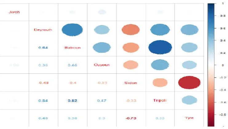
Table 16. Kendall rate between the residues of estimated GARCH processes

Simen and Sidon, where the other innovations of the stations of Beirut, Batroun Tripoli and Tire are Normal. For this reason it is necessary to apply in the following section the independence case by using the multivariate copulas. For the rest of this article, we generate a matrix called "Gvent". This matrix has seven columns and each column represents the innovations of the GARCH process at each site. The elements of the "Gvent" matrix represent the input data we use to analyze the dependence of the sites in the previous section.

Copulas dependency stations

In the previous section, we estimated seven stationary stochastic processes (GARCH) that fit the data of our seven stations (Jiyeh, Beirut, Batroun, Ouyoun EsSimen, Sidon, Tripoli and Tyre). Even if each station is modeled correctly, their joint behavior can be linked. To modelling the spatial dependency of the data, we adapt a multivariate model to the innovations of the time series. We estimate the correlations between the stations from the residuals of the estimated time series. This step will present the stations which have a geographical link according to the expression of the coefficient of correlation between the residuals. The main objective of this section is to identify the copula that describes the dependency structure between the correlated stations.

The stations that are positively linked to each other are: Batroun and Tripoli, Beirut and Batroun, Beirut and Tripoli, then Ouyoun Es Simen and Tripoli. The stationsthat are negatively related are Sidon and all other sites.First we define the using Copulas (Kalyan 2015):

 Gaussian copula: ( , … , ) =ΦΣ(Φ ( ),Φ ( ), … ,Φ ( )), where Φ and ΦΣ are respectively the cumulative density function for normal distribution (0,1), (0 ,Σ); Σ represents the correlation matrix of the margins.

 Gumbel copula: we define the function ϕ(u)=(- ln u )^θ

C(u_1,…,u_d )=-(∑_i^d▒

〖

(- lnu_i )^θ )

〗

^(1/θ) ]

Clayton copula: We define the generator function ( ) = − 1, with ∈ (0, +∞[.

( , … , ) = − + 1

/

Frank copula: We define the function ( ) = − ln ( )

( ), with ∈ (0, +∞[.

( , … , ) = −1ln [ 1 + 1

( − 1) ( − 1)]

Joe copula: we define the generator function ( ) = − ln 1 − (1 − ) with > 0.

( , … , ) = 1 − [1 − 1 − (1 − ) )

DISCUSSION

Now we can apply the test of suitability of copulas with Cramer-Von Mises and Kolmogorov-Smirnov.

Table 17. Results of the copula fit test based on the Cramer-von Mises (Sn) and the Kolmogorov-Smirnov (Tn) with a p-value rejection threshold of 5%: Beirut and Batroun stations

Copulas

Critical values P-value Critical values P-value

Gaussian 0.845403 0.959516 0 1.926238 0

Clayton 3.575376 7.184857 0 4.750594 0

Gumbel 2.787688 0.062663 0.18 0.691599 0.17

Frank 9.146738 0.679684 0 1.372695 0

Joe 4.389817 18.30545 1 5.964256 1

First, according to the p-values of the Cramer-von Mises (Sn) and Kolmogorov-Smirnov (Tn) tests, the suitability of the Gaussian and Clayton and Frank copulas to the empirical copula of the innovations is not accepted at the 5% threshold where the families of Gumbel, and Joe are accepted at the 5% threshold. We note that the Gumbel copula is significantly better than the Joe copula, since its distance to the empirical copula is lower (2.7877 vs. 4.3897 for Joe's copula).

Table 18. Results of the copula fit test based on the Cramer-von Mises (Sn) and the KolmogorovSmirnov (Tn) with a p-value rejection threshold of 5%: Tripoli and Batroun stations

Copulas

Critical values P-value Critical values P-value Gaussian 0.958878 0.149869 0.08 0.830121 0.13

Clayton 8.916911 5.382757 0 4.24299 0

Gumbel 5.458455 0.050528 0.08 0.598721 0.21

Frank 20.04181 0.408273 0 1.126818 0

Joe 9.679711 18.30545 1 5.964256 1

According to the two tests Cramer-von Mises (Sn) and Kolmogorov-Smirnov (Tn) at the 5% threshold, we accept the suitability of the copulas of Gaussian and Gumbel and Joe to the empirical copula of the innovations and we note that the Gaussian copula is significantly better than the copula of Joe and Gumbel since the distance to the empirical copula is lower (0.958878 against 9.679711 for the copula of Joe and 5.458455 for the copula of Gumbel). We do not accept the suitability of the copula Clayton and Frank.

Table 19. Results of the copula fit test based on the Cramer-von Mises (Sn) and the Kolmogorov Smirnov (Tn) with a p-value rejection threshold of 5%: Tripoli and Ouyoun Es Simen stations

Copulas

Critical values P-value Critical values P-value Gaussian 0.670951 1.150859 0 1.781753 0 Clayton 1.761006 7.829876 0 4.791284 0 Gumbel 1.880503 0.438218 0 1.238366 0

Frank 5.186759 0.74405 0 1.397748 0

Joe 2.62665 18.30545 1 5.964256 1

It is noted in Table 19 that the values for the four copulas Gaussian, Clayton, Gumbel and Frank are smaller than threshold 5% in the two tests Cramer-von Mises (Sn) and Kolmogorov-Smirnov (Tn), so we do not accept the null hypothesis of the adequacy of the copulas these copulas with the empirical copula of the innovations on the contrary one accepts it for the copula of Joe.

Table 20. Results of the copula fit test based on the Cramer-von Mises (Sn) and the KolmogorovSmirnov (Tn) with a p-value rejection threshold of 5%: Tripoli and Beirut stations

Copulas

Critical values P-value Critical values P-value Gaussian 0.752693 1.088413 0 2.090288 0 Clayton 2.371501 7.264653 0 4.872366 0 Gumbel 2.185751 0.081679 0.11 0.65344 0.27

Frank 6.567275 0.863901 0 1.677575 0

Joe 3.215188 18.30545 1 5.964256 1

At the 5% threshold we accept the suitability of the Gumbel and Joe copulas with the empirical copula of innovations with p-values> 0.05 and we note that the Gumbel copula is significantly better than the Joe copula since its distance to Copula is lower (2.185751 against 3.215188 for the copula of Joe). We do not accept the null hypothesis for the Gaussian, Clayton and Frank copula according to the two tests Cramer-von Mises (Sn) and Kolmogorov-Smirnov (Tn).

In this section we studied the bivariate copulas which are strongly dependent and we test the fit of the copulas according to the tests of Cramer-von Mises (Sn) and KolmogorovSmirnov (Tn). But what interests us in this study is to find an intermediate model that requires few parameters, while guaranteeing a satisfactory fit quality to the innovations of the multivariate variables, for this we need in order to solve this problem, for this we can interested in future research to study the Copulas“vines” where the construction of copulas in vines is based on the decomposition of a multidimensional density using the bivariate conditionals copulas.

REFERENCES

Al Zohbi, G., P. Hendrick et P. Bouillard : Evaluation du potentiel d’énergie éolienne au Liban, Revue des Energies Renouvelables Vol. 17 N°1 (2014) 83 – 96.

Allen, S. R., Hammond, G.P. and McManus, M.C., 2008. Energy analysis and environmental life-cycle assessment of a microwind turbine, Proceedings of the Institute of Mechanical Engineering, Journal of Power and Energy, Part A, Vol 222, Special Issue Paper, pp. 669-684.

Benth, J. r. a., and Benth, F. E. 2010. Analysis and modelling of wind speed in New York. Journal of Applied Statistics, 37(6), 893 - 909.

Box, G. E. P. and Cox, D. R. 1964. An analysis of transformations, Journal of the Royal Statistical Society, Series B, 26, 211-252. Dickey, D.A. W.A. Fuller, 1979. Distribution of the Estimators for Autoregressive Time Series with a Unit Root, Journal of the

American Statistical Association, 74, pp. 427-31.

Harajli, H., E. Abou Jaoudeh, J. Obeid, W. Kodieh, M.Harajli, 2011. Integrating wind energy into the Lebanese electricity system; Preliminary analysis on capacity credit and economic performance, World Engineers’ Convention 2011, September 4-9, Geneva.

Kalyan Veeramachaneni, Alfredo Cuesta-Infante, Una-May O’Reilly, Copula Graphical Models for Wind Resource Estimation, 2015

Kwiatkowski, D., P.C.B. Phillips, P. Schmidt, Y. Shin (1992): Testing the Null Hypothesis of Stationarity against the Alternative of a Unit Root, Journal of Econometrics, 54, pp. 159-178, North-Holland.

Nicola Armaroli, Vincenzo Balzani, Towards an electricity-powered world. In: Energy and Environmental Science 4, 2011. 3193– 3222, p. 3217

Oliver Grothe et Julius Schieders, 2011. Spatial dependence in wind and optimal wind power allocation: a copula based analysis, May.

Phillips, P.C.B., P. Perron, 1988. Testing for a Unit Root in Time Series Regression, Biometrika, 75, pp. 335- 346.

*******