Growth of graph powers

(1)

BIROn - Birkbeck Institutional Research Online

Pokrovskiy, Alexey (2011) Growth of graph powers. The Electronic Journal

of Combinatorics 18 (1), p. 88. ISSN 1077-8926.

Downloaded from:

Usage Guidelines:

Please refer to usage guidelines at or alternatively

(2)

Growth of graph powers

A. Pokrovskiy (LSE)

November 9, 2018

Abstract

For a graphG, itsrth power is constructed by placing an edge between two vertices if they are within distancerof each other. In this note we study the amount of edges added to a graph by taking itsrth power. In particular we obtain that either therth power is complete or “many” new edges are added. This is an extension of a result obtained by P. Hegarty for cubes of graphs.

1 Introduction

This note addresses some questions raised by P. Hegarty in [2]. In that paper he studied results about graphs inspired by the Cauchy-Davenport Theorem.

All graphs in this paper are simple and loopless. For two verticesu, v∈V(G), denote the length of the shortest path between them byd(u, v). Forv∈V(G), define itsith neighborhood

asNi(v) ={u∈V(G) :d(u, v) =i}. Therth power of a graphG, denotedGr, is constructed

fromGby adding an edge between two verticesxandywhen they are within distancerinG. Define the diameter ofG, diam(G), as the minimalr such thatGr is complete (alternatively, the maximal distance between two vertices). Denote the number of edges of Gby e(G). For v∈V(G) and a set of vertices S, defineer(v, S) =|{u∈S :d(v, u)≤r}|.

The Cayley graph of a subsetA⊆_Z_p is constructed on the vertex setZp. For two distinct

vertices x, y ∈ Zp, we define xy to be an edge whenever x −y ∈ A or y−x ∈ A. The

following is a consequence of the Cauchy-Davenport Theorem (usually stated in the language of additive number theory [1]).

Theorem 1. Let p be a prime, A a subset of Zp, and G the Cayley graph of A. Then for

any integerr <diam(G):

e(Gr)≥re(G).

If we take A to be the arithmetic progression {a,2a, . . . , ka}, then equality holds in this theorem for all r < diam(G). We might look for analogues of Theorem 1 for more general graphs G. In particular since these Cayley graphs are always regular and (whenp is prime) connected, we might focus on regular, connected G. In [2] Hegarty proved the following theorem:

Theorem 2. Suppose G is a regular, connected graph with diam(G)≥3. Then we have e(G3)≥(1 +)e(G),

with≈0.087

(3)

In other words, the cube ofGretains the original edges ofGand gains a positive proportion of new ones. In Section 3 we prove this theorem with an improved constant of = 1₆. The requirement of regularity cannot be easily dropped, as shown in [2].

Theorem 2 leads to the question of how the growth behaves for other powers of the G. Note that Theorem 2 cannot be used recursively to obtain such a result – since the cube of a regular graph is not necessarily regular. In [2] it was shown that no equivalent of Theorem 2 exists with G3 replaced by G2, and it was asked what happens for higher powers. In this note we address that question.

2 Main Result

We prove the following theorem:

Theorem 3. Suppose G is a regular, connected graph, andr≤diam(G). Then we have:

e(Gr)≥lr

3

m

−1e(G).

Proof. Let the degree of each vertex be d. Fix somev withNdiam(G)(v) nonempty.

Consider any vertexu∈V(G). Then for anyjsatisfyingd(u, v)−r < j ≤d(u, v), there is awj ∈Nj(v) such that d(u, wj)< r. For such awj, all verticesx∈N1(wj) have d(u, x)≤r.

All suchx are contained in Nj−1(v)∪Nj(v)∪Nj+1(v), hence

er(u, Nj−1(v)∪Nj(v)∪Nj+1(v))≥d. (1)

Note that eachj∈ {d(u, v)−3, d(u, v)−6, . . . , d(u, v)−3 ₁

3min{d(u, v), r}

−1

}satisfies

d(u, v)−r < j ≤ d(u, v). Summing the bound (1) over all these j, noting that any edge is

counted at most once, we obtain

er(u, N0(v)∪ · · · ∪Nd(u,v)−2(v))≥

1

3min{d(u, v), r}

d−d.

Now we sum this over allu ∈G. Note that since the edges counted above go from some Ni(v) toNj(v) with j < i, each edge is counted at most once. Also we haven’t yet counted

any of the original edges ofG, so we might as well add them. Hence

e(Gr)≥X

u∈G

er(u, N0(v)∪ · · · ∪Nd(u,v)−2(v)) +e(G)

≥X

u∈G

1

3min{d(u, v), r}

d− |V(G)|d+e(G)

=X

u∈G

1

3min{d(u, v), r}

−e(G). (2)

Obviously there was nothing particularly special aboutv. We can get a similar expresssion using v0 ∈N_diam(_G₎(v), namely

e(Gr)≥ X

u∈G

1

3min{d(u, v

0_{), r}_}

(4)

Averaging (2) and (3) we get

e(Gr)≥ 1

2

X

u∈G

1

3min{d(u, v), r}

+

1

3min{d(u, v

0_{), r}_}

d−e(G). (4)

Note that for any u∈V(G) we have

1

3min{d(u, v), r}

+

1

3min{d(u, v

0

), r}

≥lr

3

m

. (5)

This is because d(u, v) +d(u, v0) ≥d(v, v0) = diam(G) ≥ r. Putting the bound (5) into the sum (4) we obtain

e(Gr)≥ |V(G)|d

2

lr

3

m

−e(G) =

lr

3

m

e(G)−e(G).

Thus the theorem is proven.

3 Cubes

Note that forr≤6 the bounds in Theorem 3 are trivial. In particular it says nothing about the increase in the number of edges of the cube of a regular, connected graph. Such an increase was already demonstrated by Hegarty in Theorem 2. Here we give an alternative proof of that theorem, yielding a slightly better constant.

Theorem 4. Suppose G is a regular, connected graph with diam(G)≥3. Then we have

e(G3)≥

1 +1 6

e(G).

Proof. Let the degree of each vertex bed. Note that as Gis regular, and not complete, every v ∈V(G) will have a non-neighbour inG. Together with connectedness this implies that each v ∈V(G) has at least one new neighbour in G2_{. This implies the theorem for}_d_≤_{6. For the}

remainder of the proof, we assume that d >6. The proof rests on the following colouring of the edges of G: For an edgeuv in G, colour

uv red if|N1(u)∩N1(v)|>

2 3d,

uv blue if|N1(u)∩N1(v)| ≤

2 3d.

Notice that ifuvis a blue edge, then there are at least 4₃d−1 neighbours ofuinG2. This is becauseuwill be connected to everything inN1(u)∪N1(v) except itself, and|N1(u)∪N1(v)| ≥ 4

3d for uv blue. If, in addition, we have some x connected tou by an edge (of any colour),

then x will be at distance at most 3 from everything in N1(u)∪N1(v)\ {x}. Hence x will

have at least 4₃d−1 neighbours in G3. Partition the vertices ofG as follows:

B ={v∈V(G) :v has a blue edge coming out of it},

R={v ∈V(G) :v /∈B and there is au∈B such that uv is an edge},

S=V(G)\(B∪R).

By the above argument, ifv is in B∪R, then e3(v, V(G))≥ 4

(5)

will have at least one new neighbour inG2, giving e3(u, V(G))≥d+ 1. Summing these two bounds over all vertices inG, noting that any edge is counted twice, gives

2e(G3)≥

1 3d−1

|B∪R|+ (d+ 1)|S|

=

4 3d−1

|B∪R|+ (d+ 1) (|V(G)| − |B∪R|)

= 7

6d|V(G)|+ 1 3

|B∪R| −1

2|V(G)|

(d−6)

= 7

3e(G) +

1 3

|B∪R| − 1

2|V(G)|

(d−6).

Recall that we are considering the case when d > 6. Thus to prove thate(G3)≥ 7₆e(G), it suffices to show that|B∪R| ≥ 1

2|V(G)|. To this end we shall demonstrate that |S| ≤ |R|.

First however we need a proposition helping us to find blue edges in G.

Proposition 5. For any v∈V(G) there is some b∈B such thatd(v, b)≤2.

Proof. Suppose d(v, u) = 3. Then there are vertices x and y such that {v, x, y, u} forms a path between u and v. We will show that one of the edges vx, xy or yu is blue. This will prove the proposition assuming that there are any blue edges to begin with. However, it also shows the existence of blue edges because diam(G)≥3.

So, suppose that the edges vx and uy are red. Then we have |N1(v)∩N1(x)|> 2₃d, and

|N1(u)∩N1(y)|> 2₃d. Using this and |N1(u)∩N1(v)|=∅ gives

≥ |N1(x)∩N1(v)|+|N1(y)∩N1(u)|

> 4

3d.

Therefore |N1(x) ∩N1(y)| = 2d− |N1(x) ∪N1(y)| ≤ 2₃d. Hence xy is blue, proving the

proposition.

Now we will show that|S| ≤ |R|. Suppose r∈R. By the definition ofR, there is ab∈B such thatrbis an edge. This edge is neccesarily red asr /∈B. Using N1(b)⊆B∪R,we have

|N1(r)∩(B∪R)| ≥ |N1(r)∩N1(b)|> 2₃d. Hence

|N1(r)∩S| ≤

1

3d. (6)

Suppose s∈S. Proposition 5 implies that there is some r ∈R such that sr is an edge. Since sr is red, we have |N1(s)∩N1(r)|> 2₃d. Using this, the fact that N1(s)⊆R∪S, and

(6), gives

|N1(s)∩R| ≥ |N1(s)∩N1(r)∩R|

=|N1(s)∩N1(r)| − |N1(s)∩N1(r)∩S|

≥ |N1(s)∩N1(r)| − |N1(r)∩S|

> 1

(6)

Double-counting the edges betweenS andR using the bounds (6) and (7) gives a contra-diction unless|S| ≤ |R|. Therefore|B∪R| ≥ 1₂|V(G)|as required.

4 Discussion

Theorem 3 answers the question of giving a lower bound on the number of edges that are gained by taking higher powers of a graph. We obtain growth that is linear withr – just as in Theorem 1.

• The constant₁

3r

in Theorem 3 cannot be improved to something of the formλrwith

λ > 1₃. To see and consider the following sequence of graphsHr(d) asdtends to infinity:

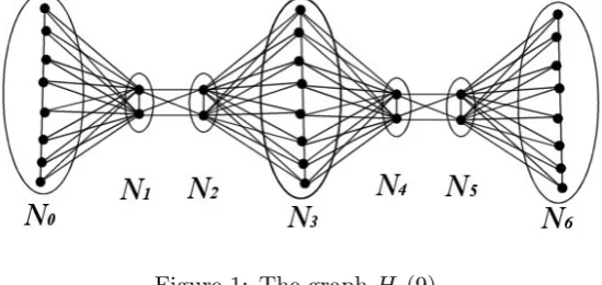
Take disjoint sets of vertices N0, ..., Nr, with|Ni|=d−1 ifi≡0 (mod 3) and|Ni|= 2

[image:6.595.165.440.322.452.2]

otherwise. Add all the edges within each set and also between neighboring ones. So if u∈Ni,v∈Nj, then uv is an edge whenever|i−j| ≤1 (see Figure 1).

Figure 1: The graph H6(9).

The number of edges inHr(d) is at least the number of edges in the larger classes which

is ₁

3(r+ 1)

d−1 2

.

The rth power Hr(d)r has less than |V(₂G)|

edges which is less than d13(r+1)e(d+3)

2

. Therefore,

lim sup

d→∞

e(Hr(d)r)

e(Hr(d))

≤ lim

d→∞ d1

3(r+1)e(d+3)

2

₁

3(r+ 1)

d−1 2

=

1

3(r+ 1)

.

The graphs Hr(d) are not regular, but ifr6≡2 (mod 3), it is possible to remove a small

(less than |V(G)|) number of edges from the graphs and make them d-regular without losing connectedness (any cycle passing through all the vertices inN1∪...∪Nr−1 would

work). Call these new graphs ˆHr(d). By the same argument as before we have

lim sup

d→∞

e( ˆHr(d)r)

e( ˆHr(d))

≤

1

3(r+ 1)

.

If r ≡2 (mod 3), a similar trick can be performed, but we’d need to start with |Ni|=

d−1 if i≡1 (mod 3) and|Ni|= 2 otherwise.

So the factor of 1₃ cannot be improved for regular graphs. All these examples are inspired by one given in [2] to show that for any there are regular graphs G with

(7)

• Despite the above example, there is certainly room for further improvement in Theorems 3 and 4. In particular, Theorem 4 doesn’t seem tight in any way. The graphs ˆHr(d)

seem to give essentially the slowest possible growth for all powers of regular graphs. Considering the graphs H3(d) leads to the conjecture of

e(G3)≥2e(G), forG regular, connected, and diam(G)≥3.

A shortcoming of Theorem 3 is that it only gives a good bound if the diameter of Gis close to r. When this is not the case, the number of edges in Gr seems to grow faster. It would be interesting to obtain a good lower bound on e(Gr) involving both r and diam(G).

• All the questions from this paper and [2] could be asked for directed graphs. In particular one can define directed Cayley graphs for a set A⊆_Z_p by lettingxy be a directed edge whenever x−y∈A. Then the Cauchy-Davenport Theorem implies an identical version of Theorem 1 for directed Cayley graphs. In this setting it is easy to show that there is growth even for the square of an out-regular oriented graphD (a directed graph where for a pair of vertices uand v,uv and vuare not both edges). In particular, we have

e(D2)≥ 3

2e(D). (8)

This occurs because every vertexvhas|Nout

2 (v)| ≥ 12|N1out(v)|in an out-regular oriented

graph. It’s easy to see that this is best possible for such graphs. One can construct out-regular oriented graphs with an arbitrarily large proportion of vertices v satisfying

|Nout

2 (v)|= 12|N1out(v)|.

However if we insist onbothin and out-degrees to be constant, (8) no longer seems tight. Such graphs are always Eulerian. In [3] there is a conjecture attributed to Jackson and Seymour that if an oriented graph D is Eulerian, then e(D2₎ _≥ ₂_e_{(D) holds. If this}

conjecture were proved, it would be an actual generalization of the directed version of Theorem 1, as opposed to the mere analogues proved above.

5 Acknowledgement

I would like to thank my supervisors Jan van den Heuvel, and Jozef Skokan for much helpful advice and remarks.

References

[1] H. Davenport,On the addition of residue classes, J. London Math. Soc., Issue 10, 30-32, (1935).

[2] P. Hegarty, A Cauchy-Davenport type result for arbitrary regular graphs. arXiv:0910.2250v2 [math.CO] , (2009).