Estimation of the Exchange Market Pressure in the EU4 Countries: A Model Dependent Approach

(1)

Estimation of the Exchange Market

Pressure in the EU4 Countries: A

Model-Dependent Approach

Stavarek, Daniel

Silesian University - School of Business Administration

September 2006

Online at

https://mpra.ub.uni-muenchen.de/7256/

(2)

ESTIMATION OF THE EXCHANGE MARKET PRESSURE IN

THE EU4 COUNTRIES: A MODEL-DEPENDENT APPROACH

Daniel Stavárek

*

Abstract

This paper estimates the exchange market pressure (EMP) on currencies of EU4 countries (Czech Republic, Hungary, Poland, Slovakia) during the period of 1993-2005. Therefore, it is one of a very few studies focused on this region and the very first paper applying the model-dependent approach to the EMP estimation on these countries. Moreover, the model proposed by Spolander (1999) is used in the paper along with quarterly data. Thus, this paper, tests the suitability of this model for the countries analyzed. Regarding the results obtained, EMP is of similar magnitude in all countries except Poland. We found that EMP was significantly lower and less volatile during the periods when a floating exchange rate arrangement was applied than in periods with fixed ex-change rates. It implies that unavoidable entry into ERM II (a quasi-fixed regime) could lead to the EMP increase during the period of the exchange rate stability criterion fulfillment. Hence, a revi-sion of the current definition and understanding of the criterion fulfillment is suggested. Since the model estimation was burdened by some factors reducing the estimates validity we also propose some modifications and extensions of the methodology applied.

Key words: exchange market pressure; model-dependent approach; EU New Member States; exchange rate stability criterion.

JEL classification: C32; E42; F31; F36.

1. Introduction

Eight countries from Central and Eastern Europe (hereafter EU8) joined the European Union (hereafter EU) in spring of 2004 and completed the transformation from centrally planned economies to market economies. Moreover, it is expected that they will also join the Eurozone and implement the euro as their legal tender. However, membership in the Eurozone is conditioned by fulfillment of the Maastricht criteria. One of which is the criterion of the national currency’s stabil-ity in the period preceding entry into the Eurozone.

This criterion is associated with specific exchange rate regime, ERM II, which must be adapted by all countries with regimes whose principles do not correspond with the ERM II’s spirit1_{. It means that all EU8 countries except for Estonia and Lithuania had or will have to modify} their exchange rate arrangement when joining ERM II2_{. The Czech Republic, Hungary and Poland} currently use flexible exchange rate arrangements. Slovakia and to a lesser extent Slovenia also maintained a flexible regime before entry into the ERM II. Such a change toward a less flexible exchange rate system could increase susceptibility of the countries to currency crises and pressures on the foreign exchange markets.

Therefore, the aim of this paper is to estimate exchange market pressure (EMP) in the Czech Republic, Hungary, Poland and Slovakia (hereafter EU4) during the period of 1993-2005. Since all countries applied both a fixed and flexible exchange rate regime, the time span chosen

*

Silesian University in Opava, Czech Republic.

Elaboration of this paper was supported by Grant Agency of the Czech Republic within the project GACR 402/05/2758 "Integration of the financial sector of the new EU member countries into the EMU"

1_{The group of incompatible regimes includes crawling pegs, free floats or managed floats without a mutually agreed}

cen-tral rate and pegs to anchors other than the euro.

2_{As of 31}st_{of December 2006, five of the EU8 (Estonia, Latvia, Lithuania, Slovakia and Slovenia) joined the ERM II.}

Nevertheless, the exchange rate regime in Latvia was very similar with the ERM II, thus the “costs” of the regime’s rear-rangement are rather marginal.

(3)

allows us to compare magnitude of tensions on the foreign exchange market in different exchange rate environments. This kind of analysis has important policy implications as the switch to a less flexible regime is unavoidable in the near future.

The paper is structured so that Section 2 describes the meaning and theoretical concept of EMP and provides a review of the relevant literature. In Section 3, the model and data used are cited; Section 4 reports the empirical results and the conclusions are presented in Section 5.

2. Exchange Market Pressure and Literature Review

2.1. Meaning and Concepts of the Exchange Market Pressure

The term “exchange market pressure” is usually related to changes of two cardinal variables describing the external sector of any economy: official international reserve holdings and the nominal exchange rate. However, the notion of EMP was more precisely defined, for the first time, in Girton and Roper (1977). In this seminal paper, the authors utilized a simple monetary model of the balance of payments to devise an index of the excess demand for money that must be relieved by either exchange rate or reserve changes to keep the money market, and hence the balance of payments, in equilibrium. The index was the simple sum of the rate of change in international reserves and the rate of change in the exchange rate. For the first time, they termed this index as EMP. However, some shortcomings can be found in the model. Since the measure is derived from a highly restrictive monetary model the for-mula cannot be applied to other models. Furthermore, a model-dependent definition is used, thus, a unique formula for EMP cannot be identified within the Girton-Roper framework.

The original concept of EMP has been modified and extended by many researchers. For example, Roper and Turnovsky (1980) and Turnovsky (1985) introduced the idea of using a small open-economy model and extended the original model by substituting the simple monetary ap-proach by an IS-LM framework with perfect mobility of capital. They allowed intervention to take the form of changes in domestic credit as well as changes in reserves. The consequence of these modifications was that the EMP was still a linear combination of the rate of change of the ex-change rate and money base but these two components were no longer equally weighted as in the Girton-Roper model.

A notable contribution to the EMP theory was provided by Weymark (1995, 1997a, 1997b, 1998). She revised the models mentioned above and introduced a more general framework in which the models are both special cases of the generalized formula. She introduced and esti-mated a parameter (conversion factor) standing for the relative weight of exchange rate changes and intervention in the EMP index. Since all previous EMP definitions stemmed from a specific model, Weymark also proposed a model-independent definition of EMP as:

The exchange rate change that would have been required to remove the excess demand for the currency in the absence of exchange market inter-vention, given the expectations generated by the exchange rate policy actu-ally implemented (Weymark, 1995, p. 278).

An extension making the simple model outlined in Weymark (1995) more realistic was introduced in Spolander (1999). He incorporated into the model a monetary policy reaction func-tion and sterilized foreign exchange intervenfunc-tion.

Many researchers have criticized the most undesirable aspect of the EMP measure, de-pendency on a particular model, and proposed some alternative approaches. A simpler and model-independent EMP measure was originally constructed in Eichengreen et al. (1996). According to this approach EMP is a linear combination of a relevant interest rate differential, the percentage change in the bilateral exchange rate and the percentage change in foreign exchange reserves. Con-trary to Weymark’s approach, the weights are to be calculated from sample variances of those three components with no need to estimate any model.

(4)

2.2. Review of Relevant Empirical Literature

Since its introduction, EMP has attracted the attention of many researchers and a great number of theoretical as well as empirical papers have been published. The empirical EMP litera-ture is bi-directionally oriented. Whereas some of the papers are directly focused on estimation of EMP in a variety of regions and countries, the second category of studies use the EMP measure as an element of subsequent analysis examining currency crises, monetary policy, foreign exchange intervention, exchange rate regime and other issues. In accordance with the geographical orienta-tion of this paper, only studies empirically analyzing EMP in EU4 are cited in the following litera-ture review.

Although EMP has been a frequently discussed and examined topic in the literature1_{one can} find a very limited number of papers focused on new EU Member States and EU4 in particular. Only four consistent studies estimating EMP in all or some of EU4 have been published to date.

The first study estimating EMP in, among others, some of EU4 (Czech Republic and Po-land) was Tanner (2002). He applied the traditional Girton-Roper model on data from 32 emerging countries and, consequently, examined the relationship between EMP and monetary policy in a vector autoregression (VAR) system. The aim was to re-examine currency crises in emerging mar-kets in 1990-2000 in a more traditional way by emphasizing the role of monetary policy at or around the time of crisis. Regarding the EMP calculated in the Czech Republic and Poland, they were modest as compared to other countries and very similar to each other. However, EMP in Po-land was twelve times higher than in the Czech Republic during the Asian in the second half of the 1990s. Tanner’s paper also provided evidence that there was a positive relationship between EMP and domestic money supply in both EU4 countries analyzed but not as significant and straight as in other countries. The only shocks to EMP can help explain monetary policy in Poland, possibly indicating sterilized intervention.

A more specific application of the Tanner (2002) approach is Bielecki (2005). The paper concentrates only on Poland from 1994-2002. The results from the VAR system analyzing the relationship between EMP and changes in domestic credit (monetary policy actions) indicate that domestic credit reacted in a counter direction to innovations to EMP. Furthermore, in his paper, Bielecki compared two EMP measures calculated under alternative methodologies (using all for-eign reserve changes and pure official forfor-eign exchange intervention data). He came to the conclu-sion that the appreciation pressure prevailed during the sample period. However, the behavior of the two indices differed to some extent, especially with events characterized by extreme EMP val-ues (July 1997, August 1998, February 1999 or July 2001). Generally, using the pure intervention data in the EMP estimation provided more realistic and robust results.

Vanneste et al. (2005) used EMP as an indicator of currency crisis and addressed the question whether currency crises in EU8 have been more frequent in fixed, intermediate or flexible exchange rate arrangements. The authors found that EMP was marginally smaller in countries and periods characterized by an intermediate exchange rate regime as compared to those with a float-ing arrangement. Regardfloat-ing EU4, the most crisis quarters (excessive EMP) occurred in Hungary during the fixed peg regime and in Poland when a crawling peg was being applied. Managed float-ing proved to be a relatively stable regime from the EMP perspective. In addition to these conclu-sions, the authors also provided evidence of high correlation between several EMP measure speci-fications with which they experimented.

Very similar conclusions were drawn in Stavárek (2005) where EMP in the Czech Repub-lic, Hungary, Poland and Slovenia in 1993-2004 is estimated. The study applied the EMP measure proposed in Eichengreen et al. (1995) and the results obtained suggest that the Czech Republic and Slovenia went through considerably less volatile development of EMP than Hungary and Poland.

Besides the focus on the still overlooked EU4 region, this paper contributes to the EMP literature in two basic aspects. First, it uses the most recent data and prolongs the period analyzed to the end of 2005. Second, this paper represents the very first application of the Weymark (1995)

1_{Some of the recent empirical studies examining EMP are Jeisman (2005) in Australia, Wyplosz (2002) in a worldwide}

(5)

and Spolander (1999) model-dependent approaches on EU4 countries. Thus, the suitability of these models for EU4 countries can be evaluated.

3. Measuring the Exchange Market Pressure: Model and Data

As mentioned previously, this study originally stems from Weymark (1995) where the following formula for EMP calculation was defined:

t t

t

e

r

EMP

=

Δ

+

η

Δ

, (1)

where

Δ

e

_t is the percentage change in exchange rate expressed in direct quotation (domestic price

for one unit of foreign currency),

Δ

r

_t is the change in foreign exchange reserves scaled by the one-period-lagged value of money base, and

η

is the conversion factor which has to be estimated from a structural model of the economy and is defined as:

t t

r

e

∂

Δ

∂

−

=

η

. (2)

The conversion factor represents elasticity that converts observed reserve changes into equivalent exchange rate units1_.

For practical estimation of EMP, the methodology introduced in Spolander (1999) was applied. Similarly with Weymark (1995), it is a model-consistent measure of EMP in the context of small open economy monetary model. However, the central bank’s monetary and foreign ex-change policies are explicitly defined, foreign exex-change intervention partly sterilized, and expecta-tions rational in the Spolander model. The model is summarized in equaexpecta-tions (3) to (9):

t t

t d

t

p

c

i

m

=

+

Δ

+

Δ

−

Δ

β

₀

β

₁

β

₂ , (3)

t t

t

p

e

p

=

+

Δ

+

Δ

* ₂

1

0

α

, (4)

t t

t

E

e

i

=

Δ

+

Δ

−

Δ

*

(

₊₁

)

, (5)

t a

t s

t

d

r

m

=

Δ

+

−

Δ

(

1 λ

)

, (6)

t t

t

p

e

r

=

−

Δ

, (5)

gap t t trend t a

t

y

p

y

d

=

γ

₀

+

Δ

+

(

1 −

γ

₁

)

Δ

−

γ

₂

Δ

, (8)

s t d

t

m

=

Δ

, (9)

where pt is domestic price level, *

t

p

is foreign price level, et denotes exchange rate (in direct

quo-tation), mt is nominal money stock (the superscript d represents the demand, and s represents the

supply), ct is real domestic income, it is nominal domestic interest rate, *

t

i

denotes nominal foreign

interest rate,

E

_t

(

Δ

e

_t₊₁

)

is expected as exchange rate change and

λ

is proportion of sterilized

intervention. All variables up to this point are expressed in natural logarithm. Next,

d

ta is

autonomous domestic lending by the central bank and rt is the stock of foreign exchange reserves,

both divided by the one period lagged value of the money base.

y

_ttrend is the long-run trend

com-ponent of real domestic output yt and

gap t

y

is the difference between yt and

trend t

y

. The sign

Δ

naturally denotes change in the respective variable.

Equation (3) describes changes in money demand as a positive function of domestic infla-tion and changes in real domestic income and a negative funcinfla-tion of changes in the domestic inter-est rate. Equation (4) defines the purchasing power parity condition attributing the primary role in

1_{There is an assumption that all intervention takes the form of purchases or sales of foreign exchange reserves. When, in}

(6)

domestic inflation determination to exchange rate changes and foreign inflation. Equation (5) de-scribes uncovered interest rate parity. Equation (6) suggests that changes in the money supply are positively influenced by autonomous changes in domestic lending and unsterilized changes in the stock of foreign reserves. Equation (7) states that changes in foreign exchange reserves are a func-tion of the exchange rate and a time-varying response coefficient

p

_t. Equation (8) describes the evolution of the central bank’s domestic lending. Whereas domestic inflation and changes in trend real output changes are positive determinants of the domestic lending the gap between real output and its trend has a negative impact on domestic lending activity. Equation (9) defines a money market clearing condition that assumes money demand to be continuously equal to money supply.

By substituting equations (4) and (5) into equation (3) and substituting equation (8) into equation (6) and then using the money market clearing condition in equation (9) to set the resulting two equations equal to one another, it is possible to obtain the following relation:

2 2 1

1

2 ( ) (1 )

β α γ λ β + Δ − + Δ + =

Δ t t+ t

t

r e

E X

e , (10)

where * 2 1 2 * 1 1 0 0 1

0 t t

gap t t trend

t

y

p

y

c

i

X

=

γ

−

γ

α

−

β

+

Δ

−

γ

α

Δ

−

γ

−

β

Δ

+

β

Δ

(11) and the elasticity needed to calculate EMP in equation (1) can be found as:

2 2 1 ) 1 (

β

α

γ

λ

η

+ − − = Δ ∂ Δ ∂ − = t t r e . (12)

The samples of data used in this paper cover the period of 1993:1 to 2005:4 yielding 52 quarterly observations for all EU4 countries. The data were predominantly extracted from the IMF’s International Financial Statistics and the Eurostat’s Economy and Finance database. The missing observations in the time series were replenished from databases accessible on the EU4 central banks’ websites1_{. The detailed description of all data series and their sources is presented in} Appendix. Nevertheless, a brief overview of the data used is provided here for better understand-ing of the model described above.

We used nominal bilateral EU4 national currencies exchange rates against the euro (et).

The exchange rates prior to 1999 were obtained using the irrevocable conversion rate of the Ger-man mark to the euro. The domestic (it) as well as foreign interest rate (

*

t

i

) are represented by the 3-month money market rates in EU4 countries and the Eurozone. The M1 monetary aggregate was employed as the domestic money stock (mt). The domestic (pt) and foreign price levels (

*

t

p

) are proxied by the respective consumer price index. As the level of domestic output (yt) we applied the

gross domestic product (GDP). The gross national income (ct) was derived by adding the net

in-come from abroad to GDP. The domestic money base (Bt) and total reserves minus gold (rt) were

also included in the EMP estimation.

4. Estimation of the Exchange Market Pressure

As is evident from the model presented in the previous section, the EMP estimation (1) must be preceded by the calculation of the conversion factor

η

(2, 12). This step is, however,

re-quired to obtain values of the sterilization coefficient

λ

(6), the elasticity of the money base with respect to the domestic price level

γ

₁ (8), the elasticity of the domestic price level with respect to

the exchange rate

α

₂ (4), and the elasticity of the money demand with respect to the domestic

interest rate

β

2 (3).

More precisely, the parameter estimates are obtained by estimating the following three equations.

(7)

t t t

t

p

c

i

m

−

Δ

=

β

₀

+

β

₁

Δ

−

β

₂

Δ

+

ε

₁_,

Δ

, (13)

t t t

t

p

e

p

* ₂ ₂_,

1

0

α

ε

α

+

Δ

+

Δ

+

=

Δ

, (14)

t gap t t t t trend t t t

t

_r

_y

_p

_r

_p

_y

B

, 3 2 1 0 1

ε

γ

λ

γ

+

Δ

+

Δ

+

=

Δ

−

Δ

−

Δ

−

Δ

−

. (15)

Equations (13) and (14) are obtained directly from equations (3) and (4). Equation (15) is derived by substitution of (7) into (5) and noting that change in money supply equals the change in

money base 1 −

Δ

t t

B

assuming the money multiplier to be constant.

One can distinguish two types of variables included in the model: endogenous and

exoge-nous. The endogenous variables are

Δ

m

_t ,

Δ

p

_t ,

Δ

e

_t ,

Δ

i

_t , 1 −

Δ

t t

B

and

Δ

r

_t . The exogenous

variables are

Δ

c

_t ,

Δ

p

_t*,

Δ

i

_t*,

Δ

y

_ttrend and

Δ

y

_tgap. Despite the fact that

Δ

e

_t does not appear on the left-hand side of any of the equations, it is the endogenous variable because the exchange rate is clearly the variable determined by this model.

The model is estimated using the two-stage least square regression technique (2SLS). The main reason is that the endogenous variables are on both sides of equations (3)-(9). It means that in each equation having endogenous variables on the right-hand side, these variables are likely to correlate with the disturbance term. Thus, using the ordinary least square method would lead to biased estimates. On the other hand, the three-stage least square method was not chosen because of the limited size of the dataset used (small number of observations).

The 2SLS used requires the incorporation of instruments (variables uncorrelated with the disturbance term) into the estimation. Thus, the first empirical step of the analysis was to find ap-propriate instruments. For this purpose we run the first stage regressions on endogenous variables having all possible instruments as regressors. As possible instruments we set the contemporaneous and one-quarter lagged values of exogenous variables and one-quarter lagged values of all en-dogenous variables. Finally, the regressors with sufficient statistical significance were selected as instruments. This procedure was carried out for all countries and equations of the model.

The next aspect which had to be assessed is the stationarity of regressors. This feature is essential for all regression models. We applied Phillips-Perron and Augmented Dickey-Fuller tests to examine the stationarity of the time series used. Uniform outcomes of both tests were necessary for the final conclusion about the (non)stationarity of each time series. According to the character of each time series we tested the stationarity with a linear trend and/or intercept or none of them. To conserve space the stationarity tests’ results are not reported here but they allow us to conclude that the first differences of all time series are stationary. Thus, they can be used in estimation of all equations of the model1_.

The 2SLS estimation results are presented in Tables 1 to 3, individually for each equation. The tables also contain the list of instruments and results of some diagnostic tests. We applied Jar-que-Berra (J-B) indicator to assess normality of the residuals distribution, Breusch-Godfrey Lan-grange Multiplier (LM) to test serial correlation and White test to check heteroscedasticity. All LM tests were run with four lags. The tests indicated evidence of serial correlation in residuals from the equations and the potential heteroscedasticity was also identified in some cases. Therefore, we corrected the standard errors of parameter estimates by the Newey-West procedure. Even more frequently, the residuals seem to be non-normally distributed. Therefore although the t-statistics can be misleading, this does not reduce the validity of the parameter estimates2_{. According to the}

1_{The percentage change in money base is a naturally flow variable and, thus, already differenced and stationary. Likewise,}

ytgap is stationary on level in all countries because of its construction.

2_{Since different equation specifications have different instruments, R}2_{for 2SLS can be negative even if a constant is used}

(8)

model specification the parameters

β

₁,

α

₁, and

α

₂ should be positive and

β

₂,

γ

₁,

γ

₂, and

λ

[image:8.595.98.498.148.424.2]

should be negative. Since

λ

is a fraction, its absolute value should be between zero and one.

Table 1

Estimates of equation (13)

Czech Republic Hungary

Instruments: trend t y₋₁

Δ Δrt−1 Δit−1

gap t y Δ * 1 −

Δpt Instruments: Δct

*

t p

Δ Δit−1

trend t y₋₁

Δ

Param. Estim. St. er. Prob. Param. Estim. St. er. Prob.

β0 0.0014 0.0036 0.6945 β0 -0.0052 0.0021 0.0152

β1 0.0161 0.7711 0.9834 β1 0.4843 0.2290 0.0397

β2 -0.0434 0.0161 0.0096 β2 -0.0216 0.0208 0.3039 R2=0.0792, SEE=0.0098, DW=1.9422 R2=0.1237, SEE=0.0092, DW=1.4480

J-B=30.721 (0.0000), LM=4.7744 (0.3112) WHITE=23.724 (0.0002)

J-B=4.3279 (0.1149), LM=20.689 (0.0004) WHITE=5.0859 (0.4055)

Poland Slovakia

Instruments: trend t y₋₁

Δ Δet−1 Δit−1

*

t p

Δ Δct−1 Instruments: Δct−1 *

1

−

Δpt Δmt Δpt−1 Δit−1

β0 0.0013 0.0023 0.5684 β0 0.0022 0.0039 0.5650

β1 0.2281 0.1430 0.1174 β1 -0.6005 0.5969 0.3195

β2 -0.0873 0.0310 0.0070 β2 -0.0781 0.0573 0.1793 R2=-0.2601, SEE=0.0102, DW=2.3324 R2=-0.8812, SEE=0.0177, DW=1.6388

J-B=0.8370 (0.6580), LM=7.5026 (0.1116) WHITE=24.305 (0.0002)

J-B=48.437 (0.0000), LM=3.7018 (0.4479) WHITE=2.3160 (0.8039)

Source: Author’s calculations.

The estimations of equation (13) provide mediocre results. The parameters β₂ necessary for the conversion factor calculation are correctly signed in all EU4. However, they are statistically significant only in the Czech Republic and Poland. One can see some evidence of non-normal dis-tribution (Czech Republic, Slovakia), serial correlation (Hungary) and heteroscedasticity (Czech Republic and Poland).

Table 2

Instruments: *

t p

Δ trend t y−₁

Δ *

1

−

Δi_t Δet−₁ Instruments:

*

t p

Δ trend t y−₁

Δ Δc_t Δpt−₁

α0 0.0022 0.0017 0.2061 α0 0.0005 0.0011 0.6424

α1 1.3408 1.1845 0.2634 α1 2.9075 0.8607 0.0015

α2 0.8385 0.3671 0.0269 α2 0.9514 0.1541 0.0000 R2=-2.9906, SEE=0.0059, DW=1.7739 R2=0.3453, SEE=0.0047, DW=1.8062

J-B=7.9568 (0.0187), LM=7.7211 (0.1023) WHITE=40.979 (0.0000)

[image:8.595.100.497.558.690.2]

(9)

Table 2 (continued)

Poland Slovakia Instruments: *

t p

Δ Δet−₁ Δit−1 Δpt−1 Δct−1 *

1

−

Δp_t Instruments: *

t i

Δ Δet−₁

gap t y Δ trend t y Δ * 1 −

Δp_t Param. Estim. St. er. Prob. Param. Estim. St. er. Prob.

α0 -0.0005 0.0022 0.8207 α0 0.0028 0.0031 0.3617

α1 3.8073 1.5226 0.0159 α1 0.9512 2.4477 0.6993

α2 0.2006 0.0355 0.0000 α2 0.6360 0.3155 0.0496 R2=0.1221, SEE=0.0066, DW=1.6167 R2=-1.0946, SEE=0.0054, DW=1.9761

J-B=0.7071 (0.7021), LM=8.4398 (0.0767) WHITE=3.9881 (0.5511)

J-B=2.0481 (0.3591), LM=5.1151 (0.2756) WHITE=14.169 (0.0146)

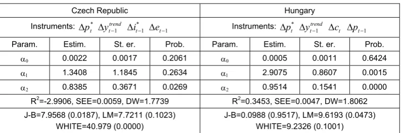
[image:9.595.100.498.93.206.2]

In the estimations of equation (14) we obtained very good results. The signs of all pa-rameters are consistent with the theoretical assumptions and important

α

₂ parameters are signifi-cantly different from zero in all countries. On the other hand, however, only error terms in the Pol-ish equation seem to pass the standard diagnostic tests completely. Furthermore, one can see a substantially lower elasticity of the domestic price level with respect to the exchange rate (

α

₂) in Poland than in other EU4. Although it is not directly linked with the EMP estimation, it is worth-while to point out a general feature of relatively high elasticity of the domestic price level with respect to the foreign inflation. One can find that quite common in small and open economies dur-ing the transition period.

Table 3

Instruments: *

t p

Δ gap

t y

Δ Δrt−1

*

t i

Δ Δit−1 trend t y−1

Δ Instruments: gap t y

Δ *

1

−

Δit Δct−1

gap t y−1

Δ Δit−1

γ0 -0.0007 0.0024 0.7634 γ0 0.0007 0.0049 0.5755

λ -0.7743 0.1835 0.0001 λ -0.5133 0.2911 0.0575

γ1 -1.0995 1.2202 0.3722 γ1 -1.7329 0.9774 0.0829

γ2 0.0006 0.0007 0.3727 γ2 0.0001 3.4E-05 0.0024 R2_{=0.4316, SEE=0.0198, DW=2.1887} _R2_{=0.5935, SEE=0.0132, DW=2.4603}

J-B=129.37 (0.0000), LM=0.9345 (0.9195) WHITE=43.358 (0.0000)

J-B=26.582 (0.0000), LM=9.4808 (0.0501) WHITE=11.339 (0.2531)

Poland Slovakia Instruments:

1

−

Δmt

*

t p

Δ trend

t

y−1

Δ *

1

−

Δpt gap t y

Δ Instruments: trend t y−1

Δ Δct

* 1

−

Δit gap t y−1

Δ Δit−1

γ0 -0.0043 0.0035 0.2284 γ0 0.0083 0.0074 0.2693

λ -1.4333 0.3308 0.0001 λ -0.9005 0.1252 0.0000

γ1 1.5112 1.1929 0.2116 γ1 -3.1911 2.3325 0.1779

γ2 -0.0002 0.0009 0.8194 γ2 -0.0007 0.0021 0.7312 R2=0.7343, SEE=0.0231, DW=2.4286 R2=0.9512, SEE=0.0224, DW=2.4020

J-B=9.6651 (0.0080), LM=8.2987 (0.0812) WHITE=10.243 (0.3311)

J-B=2.8966 (0.2349), LM=9.2211 (0.0558) WHITE=5.1728 (0.8189)

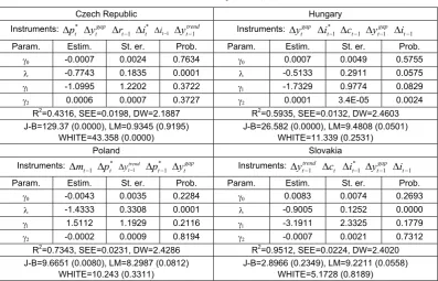
[image:9.595.99.497.379.634.2]

(10)

λ

exceeded the upper margin of the potential interval from zero to one. Moreover,

λ

in Hungary and

γ

₁ in all EU4 are statistically insignificant at the 5% level. Neither the performance of the

elasticities of the money base with respect to the domestic output gap (

γ

₂) are significant. Accord-ing to Spolander (1999, p. 72) this problem stems from different specification of the equation and, unfortunately, it is a common drawback of many studies of monetary policy rules and reaction functions. As stated in McCallum (1997, p. 8), there has been much debate on the subject of mone-tary policy rules but the appropriate specification of a model suitable for the analysis of monemone-tary policy rules does not exist.

The parameter estimates of the sterilization coefficients

λ

in all EU4 do not significantly differ from minus unity, which implies full sterilization1_{. However, the EU4 central banks have} never publicly declared that all foreign exchange intervention has no impact on the money base. Hence, we assume that the parameter estimates of

λ

indicate less than full sterilization. This as-sumption is in accordance with the practice of central banks from developed countries which usu-ally sterilize their intervention partiusu-ally rather than fully.

Table 4

Estimates of conversion factors

Czech Republic Hungary Poland Slovakia

1.8380229 0.9060151 -11.273278 0.8999273

Table 4 summarizes estimates of the conversion factors

η

calculated for all countries us-ing equation (12). Due to non-standard results of the estimation of equation (15) in Poland, the Polish conversion factor differs substantially from other factors in magnitude as well as sign. The extraordinary value of Polish

η

is subsequently transmitted to EMP whose extent will not corre-spond with the EMP scale in other EU4.

The EMP development in all EU4 countries analyzed is graphically presented in Figures 1 to 4. To analyze EMP correctly it is necessary to remember some elementary facts. First, a nega-tive value of EMP indicates that the currency is under general pressure to appreciate. On the con-trary, positive EMP shows that the currency is pressured to depreciate. Second, the value of EMP represents the magnitude of the foreign exchange market disequilibrium which should be removed by a respective change of the exchange rate.

[image:10.595.200.389.496.638.2]

Source: Author’s calculation.

Fig. 1. Exchange market pressure in Czech Republic

1_{The Wald test of the null hypothesis}

λ

_{=-1 resulted in the following F-statistics and probabilities. Czech Republic:}

(11)

[image:11.595.202.389.86.226.2]

Fig. 2. Exchange market pressure in Poland

[image:11.595.208.390.278.417.2]

Fig. 3. Exchange market pressure in Hungary

Fig. 4. Exchange market pressure in Slovakia

[image:11.595.206.390.468.609.2]

(12)

[image:12.595.96.500.154.266.2]

sections, thus allowing the distinguishing of different exchange rate arrangements applied in EU4 during the period examined. See Table 5 for the basic descriptive statistics of EMP.

Table 5

Descriptive statistics of exchange market pressure

Mean 0.016407 0.009117 -0.221316 0.021629

Median 0.006589 0.007108 -0.100831 0.007484

Maximum 0.116360 0.054982 0.327037 0.233425

Minimum -0.034128 -0.019079 -1.292694 -0.068756 Standard dev. 0.034257 0.016044 0.388165 0.052023

Upper limit 0.067793 0.033183 0.360931 0.099664

Lower limit -0.034979 -0.014948 -0.803564 -0.056406

One can find the EMP development in EU4 as alike in many aspects. The first three years were characterized by many episodes of excessive EMP and its high volatility. The EMP estimates suggest that there was a general pressure on EU4 currencies to depreciate. The principal exception was Poland whose EMP measurements surpassed 120% on the appreciation side for three times in 1993-1995. It is very hard to believe that the magnitude of money market disequilibrium would be so enormous that the Polish zloty should have appreciated by 120% in order to remove that dis-equilibrium noting the still starting stage of the transformation process. Moreover, Vanneste et al. (2005) as well as Bielecki (2005) obtained considerably different (and more realistic) estimations of EMP in Poland in that period.

It is worthwhile to remember that all EU4 countries applied some version of fixed exchange rate regime in 1993-1995. Furthermore, the Czech Republic and Slovakia started their existence in January 1993 after the split of former Czechoslovakia. The related currency separation, launch of new currencies, establishment of new central banks, and formation of new monetary policies had an obvious impact on data used in the estimation and consequently on the EMP figures.

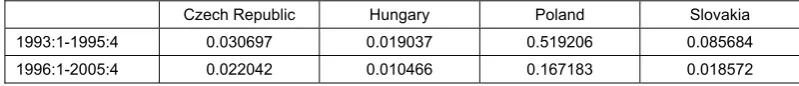
Since 1996, EMP developed more smoothly and free of any abnormal fluctuations. It can be documented by the analysis of EMP standard deviations from both periods (see Table 6). The standard deviations in 1996-2005 were substantially lower than in period of 1993-1995. There was only one example of breaching the corridor’s margin in the Czech Republic and Hungary after 1995. In 2002:2, the EMP in the Czech Republic was 7.09% forcing the koruna (CZK) to depreci-ate. This reflected the necessity for a correction after the previous long-lasting appreciation and peaking at the historic high. In Hungary, on the other hand, the EMP in 2002:1 was -1.91% sug-gesting a pressure on the forint (HUF) to appreciate. A high (not excessive) EMP also occurred at the end of 2002. HUF was under speculative attack on the upper edge of the band which culmi-nated in devaluation of the central parity. Whereas the depreciation pressure prevailed on HUF and Slovak koruna the proportion of appreciation-pressure and depreciation-pressure quarters was more balanced in the case of CZK in 1996-2005.

Table 6

Standard deviations of exchange market pressure

1993:1-1995:4 0.030697 0.019037 0.519206 0.085684 1996:1-2005:4 0.022042 0.010466 0.167183 0.018572

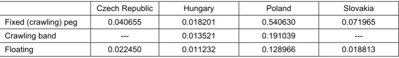
[image:12.595.96.496.644.687.2]

(13)

[image:13.595.100.496.222.280.2]

One of the aims of the paper is to compare EMP in various exchange rate arrangements in EU4 keeping in mind the necessity to enter into ERM II (a quasi-fixed regime with a fluctuation band) and fulfill the exchange rate stability criterion in EU4 in the near future. The results clearly suggest that EMP during the floating-regime period was very stable in all EU4 and the excessive deviations of EMP occurred sporadically. On the contrary, as already mentioned, the periods of fixed arrangement witnessed numerous episodes of surpassing the 1.5 multiple of standard tion level along with the more volatile development. The comparison of the EMP standard devia-tions calculated over the periods with particular exchange rate regime is provided in Table 7.

Table 7

Standard deviations of exchange market pressure

Fixed (crawling) peg 0.040655 0.018201 0.540630 0.071965 Crawling band --- 0.013521 0.191039 ---

Floating 0.022450 0.011232 0.128966 0.018813

These findings would cast serious doubt on the European Commission’s requirement that EU4 must participate in ERM II without substantial tensions on the exchange rates. The doubt gains importance if the actual European authorities’ position to the fulfillment of the exchange rate stability criterion is considered as decisive. When all relevant statements and declarations of the ECB, European Commission and Ecofin Council are summarized and combined with the ap-proaches to the criterion assessments applied in the past, we can consider the use of the ERM II standard fluctuation band of ± 15% as highly improbable. On the contrary, the authorized fluctua-tion margin is likely to be asymmetric with the limits of 15% on the appreciafluctua-tion side and 2.25% on the depreciation side.

Although EMP fluctuated predominantly within this narrow band in EU4 in the last four years there was no a priory set limit of maximal appreciation or depreciation whose exceeding could be punished. Such circumstances could contribute to the emergence of a speculative attack on EU4 currencies when participating in ERM II. Thus, the paper’s findings support some revision of the current definition and understanding of the exchange rate stability criterion fulfillment. We suggest a complete abolishment of the ERM II and its meaningless standard fluctuation band of ± 15% around the central parity and its substitution by the ex-post assessment of the criterion ful-fillment. The modifications proposed could reduce the possibility of shock after the substantial shift in the exchange rate policy from the floating to the quasi-fixed exchange rate regime.

Owing to some factors the EMP estimates presented and discussed previously must be viewed with some degree of skepticism. There are several drawbacks which must be taken into account when interpreting the results obtained. First, many parameter estimates required for calcu-lation of the conversion factor and EMP are statistically insignificant. It can be attributed to either wrong specification of the model or some problems with estimation procedure or data used. Sec-ond, the parameter estimates are sensitive to the choice of instruments and even small changes in the parameters’ values have a considerable impact on EMP. Third, the sterilization coefficient in none of EU4 is significantly different from minus unity which indicates full sterilization. Fourth, EMP in all countries behaved almost absolutely parallel to changes in reserves during the entire period1_{. It implies a frequent application of the central bank official intervention even in the} envi-ronment of floating exchange rate regime. The reality in many EU4 was, however, different.

These limitations should be eliminated in future research. We recommend use of the pure foreign exchange intervention data as an alternative to the change in reserves. It could lead to more plausible results as evident in Bielecki (2005). The model could also be extended by the possibility

(14)

of indirect intervention operating through changes in domestic lending or the domestic interest rate. To obtain comparable results, we suggest applying a model-independent approach originated by Eichengreen et al. (1996). The main advantage of this approach is the greater emphasis put on the interest rate differential, which has often been identified as a factor of exchange rate determi-nation in EU4.

5. Conclusion

In this paper, we estimated EMP for the EU4 currencies against the euro exchange rate over the period of 1993-2005. We applied the Spolander (1999) model based on the Weymark (1995) model-dependent approach. Although there are some concerns about the validity of the parameter estimates and consequently the EMP measures we can draw several conclusions. The EMP in the Czech Republic, Hungary and Slovakia is of similar magnitude. Whereas a deprecia-tion pressure prevailed on the Hungarian forint and the Slovak koruna, no dominance of any direc-tion of the pressure can be found in the case of the Czech koruna. The estimates of the Polish EMP are burdened by substantial statistical insignificance. The results obtained suggest that EMP in EU4 decreased over time and was substantially lower and less volatile during the periods of float-ing exchange rates than in the environment of fixed exchange rate regime. It implies that although EMP in all EU4 was relatively small and stable in the last four years, a shift to the quasi-fixed ERM II and start of the exchange rate stability criterion fulfillment could evoke EMP to grow to excessive levels. Thus, we suggest revision of the definition and understanding of the exchange rate stability criterion in favor of the ex-post assessment of the fulfillment instead of the applica-tion of any kind of fluctuaapplica-tion band. Addiapplica-tionally, due to inconsistent results of the model estima-tion, we conclude that the Spolander (1999) model in its pure version is not fully suitable for EU4 and we recommend some extensions and propose further steps for future research.

References

1. BIELECKI, S. (2005). Exchange market pressure and domestic credit evidence from Poland.

The Poznan University of Economics Review, vol.5, 2005, pp. 20-36.

2. EICHENGREEN, B., ROSE, A.K., WYPLOSZ, C. (1996). Exchange Market Mayhem: The An-tecedents and Aftermath of Speculative Attacks. Economic Policy,vol. 10, 1996, pp. 251-312. 3. GIRTON, L., ROPER, D. (1977). A Monetary Model of Exchange Market Pressure

Applied to the Postwar Canadian Experience. American Economic Review,vol. 67, 1977, pp. 537-548.

4. JEISMAN, S. (2005). Exchange Market Pressure in Australia. Quarterly Journal of Business and Economics, vol. 44, 2005, pp. 13-27.

5. KAMALY, A., ERBIL, N. (2000). A VAR Analysis of Exchange Market Pressure: A Case Study for the MENA Region. Economic Research Forum Working Paper 2025.

6. KOHLSCHEEN, E. (2000). Estimating Exchange Market Pressure and Intervention Activity.

Banco Central do Brasil Working Paper No. 9.

7. MCCALLUM, B.T. (1997). Issues in the Design of Monetary Policy Rules. Working Paper No. 6016. National Bureau of Economic Research.

8. PENTECOST, E.J., VAN HOOYDONK, C., VAN POECK, A. (2001). Measuring and Esti-mating Exchange Market Pressure in the EU. Journal of International Money and Finance, vol. 20, 2001, pp. 401-418.

9. ROPER, D., TURNOVSKY, S.J. (1980). Optimal Exchange Market Intervention in a Simple Stochastic Macro Model. Canadian Journal of Economics, vol. 13, 1980, pp. 296-309. 10. SPOLANDER, M. (1999). Measuring Exchange Market Pressure and Central Bank

Interven-tion. Bank of Finland Studies E:17.

11. STAVÁREK, D. (2005). Exchange Market Pressure in New EU-member Countries. In:

(15)

12. TANNER, E. (2002). Exchange Market Pressure, Currency Crises, and Monetary Policy: Additional Evidence from Emerging Markets. Working Paper WP/02/14. International Monetary Fund.

13. TURNOVSKY, S.J. (1985). Optimal Exchange Market Intervention: Two Alternative Classes of Rules, in BHANDARI, J.S. (ed.) Exchange Rate Management Under Uncertainty.

Cambridge: MIT Press, 1985.

14. VANNESTE, J., VAN POECK, A., VEINER, M. (2005). Exchange rate regimes and ex-change market pressure in accession countries. Working paper 2004012. University of Antwerp, Department of Economics.

15. WEYMARK, D.N. (1995). Estimating Exchange Market Pressure and the Degree of Ex-change Market Intervention for Canada. Journal of International Economics, vol. 39, 1995, pp. 273-295.

16. WEYMARK, D.N. (1997a). Measuring the Degree of Exchange Market Intervention in a Small Open Economy. Journal of International Money and Finance, vol. 16, 1997, pp. 55-79. 17. WEYMARK, D.N. (1997b). Measuring Exchange Market Pressure and Intervention in

Inter-dependent Economy: A Two-Country Model.” Review of International Economics, vol. 5, 1997, pp. 72-82.

18. WEYMARK, D.N. (1998). A General Approach to Measuring Exchange Market Pressure.

Oxford Economic Papers, vol. 50, 1998, pp. 106-121.

19. WYPLOSZ, C. (2002). How Risky is Financial Liberalization in the Developing countries.

(16)

Appendix: Data description

All data are on quarterly basis and cover the period of 1993:1-2005:4

Bt EU4 national money base

Obtained from IMF’s International Financial Statistics (IFS) line 14 (Reserve money) and then logged.

ct EU4 Gross national income

Derived by adding the net income from abroad to Gross domestic product (IFS line 99B). In national accounts statistics, the total of rents, interest, profits and dividends plus net current transfers is shown as “net income from abroad”. It was obtained from IFS by differencing current account balance (IFS line 78ALD) and balance on goods and services (IFS line 78AFD). Logged values. et Nominal bilateral exchange rate of EU4 currencies vis-à-vis euro in direct quotation (number of EU4

currency units for one euro)

Obtained from Eurostat’s Economy and finance database (EEF) section Exchange rates and Interest rates, line Euro/ECU exchange rates – Quarterly data. Logged values.

it* Eurozone 3-month money market interest rate

Obtained from EEF section Exchange rates and Interest rates, line Money market interest rates – Quarterly data, series MAT_M03.

it EU4 national 3-month money market interest rate

Obtained from EEF section Exchange rates and Interest rates, line Money market interest rates – Quarterly data, series MAT_M03.

mt EU4 national M1 monetary aggregate

Obtained from IFS line 34..B (Money, Seasonally Adjusted) and then logged. pt

*

Eurozone Harmonized indices of consumer prices

Obtained from EEF section Prices, line Harmonized indices of consumer prices – Monthly data (index 2005=100). Converted from monthly to quarterly data by averaging the three monthly figures and then logged.

pt EU4 national Harmonized indices of consumer prices

Obtained from EEF section Prices, line Harmonized indices of consumer prices – Monthly data (index 2005=100). Converted from monthly to quarterly data by averaging the three monthly figures and then logged.

rt EU4 national official reserves holdings

Obtained from IFS line 1L.D (Total Reserves Minus Gold) converted to national currency using nominal bilateral exchange rate vis-à-vis US dollar (IFS line AE) and then logged.

yt EU4 national Gross domestic product

Obtained from IFS line 99B (Gross Domestic Product) and then logged. yttrend Long-run component of yt