Munich Personal RePEc Archive
Can Panel Data Really Improve the
Predictability of the Monetary Exchange
Rate Model?
Westerlund, Joakim and Basher, Syed A.
York University
20 December 2006
Online at
https://mpra.ub.uni-muenchen.de/1229/
Can Panel Data Really Improve the Predictability of
the Monetary Exchange Rate Model?
∗Joakim Westerlund† and Syed A. Basher‡
December 11, 2006
Abstract
A common explanation for the inability of the monetary model to beat the random walk in forecasting future exchange rates is that conventional time series tests may have low power, and that panel data should generate more powerful tests. This paper provides an extensive evaluation of this power argument to the use of panel data in the forecasting context. In particular, by using simulations it is shown that although pooling of the individual prediction tests can lead to substantial power gains, pooling only the parameters of the forecasting equation, as has been suggested in the previous literature, does not seem to generate more powerful tests. The simulation results are illustrated through an empirical application.
JEL Classification: C15; C32; C33; F31; F47.
Keywords: Monetary Exchange Rate Model; Forecasting; Panel Data; Pooling; Bootstrap.
1
Introduction
Since the seminal article by Meese and Rogoff (1983), showing that forecasts based on the monetary model could not outperform those of a simple ran-dom walk, exchange rate predictability has been a major enterprise among
∗The authors would like to thank Massimilliano Marcellino and one anonymous referee
for many valuable comments and suggestions. The first author would also like to thank the Maastricht Research School of Economics of Technology and Organizations for its hospitality during a visit at the Depertment of Quantitative Economics at the University of Maastricht, where a part of this paper was written. Thank also to the Jan Wallander and Tom Hedelius Foundation for financial support under research grant number W2006-0068:1. The usual disclaimer applies.
†Corresponding author: Department of Economics, Lund University, P. O. Box 7082,
S-220 07 Lund, Sweden. Telephone: +46 46 222 8670; Fax: +46 46 222 4118; E-mail address: [email protected].
‡Department of Economics, York University, Toronto, ON, M3J 1P3, Canada. E-mail
economists. Because of its strong intuitive appeal, and because monetary fun-damentals are likely to influence exchange rate changes, the poor forecasting performance of the monetary model has puzzled economic theoreticians for many years. It has also spawned an enormous amount of empirical research dedicated to explaining why the random walk is so difficult to beat in terms of forecasting accuracy.
The single most noticeable study within this latter field of research is that of Mark (1995), who tested the predictive ability of the monetary model rel-ative to the random walk using quarterly data for Canada, Germany, Japan and Switzerland covering the period 1973:Q2 to 1991:Q4. To evaluate the forecasts, Mark (1995) used both the Theil U statistic and the S statistic of Diebold and Mariano (1995). Unfortunately, tests such as these are compli-cated by various econometric problems, such as overlapping observations and bias, which make inference unreliable. To account for this, Mark (1995) sug-gested bootstrapping the tests under the null hypothesis of no predictability. Based on the bootstrapped tests, the author found strong evidence favoring the forecast accuracy of the monetary model relative to the random walk. The author also found that the evidence tended to increase with the forecasting horizon.
The positive empirical results, coupled with the innovative use of the boot-strap, caused renewed interest in the monetary model and its predictive ability. However, although some confirmatory evidence were found, it was soon clear that the study of Mark (1995) suffered from several econometric deficiencies that made the conclusions highly questionable.
For example, the Mark (1995) bootstrap assumed that the exchange rate and monetary fundamentals were cointegrated as predicted by the monetary model. Berben and van Dijk (1998) proved that the failure of this assump-tion rendered the estimated forecasting equaassump-tion biased in such a way that predictability would be found even though none existed. They also found that the bias was increasing in the forecasting horizon, which explained why Mark (1995) found more predictive evidence at longer horizons. Similarly, Berkowitz and Giorgianni (2001) derived bootstrap critical values for the U
and S statistics under the assumption of no cointegration, and showed that falsely imposing cointegration can make the tests biased toward rejecting the null of no predictability. The authors also demonstrated that the evidence of predictability found by Mark (1995) was weakened when the critical values were generated under the null of no cointegration.
Based on a less restrictive data generating process and an updated data set, Kilian (1999) found only weak evidence in favor of exchange rate predictability. The author also showed that the better predictability at long horizons found by Mark (1995) could be explained in terms of larger size distortions rather than better power, which corroborated the Berben and van Dijk (1998) results. The pioneering study of Mark (1995), and the critique that followed, have left the predictability of exchange rates an open question. Starting with Groen (2000) and Mark and Sul (2001), this has inspired several authors to employ larger panel data sets in order to illuminate the issue. Mark and Sul (2001) used quarterly observations for 19 countries between 1973:Q1 and 1997:Q1, and found support in favor of cointegration for all countries regardless of the choice of numeraire country considered. The authors then tested the pre-dictability of the monetary model using bootstrap inference with the coin-tegration restriction superimposed. In so doing, they assumed that the pa-rameters of the forecasting equation could be pooled, which should enable better estimation precision. Based on these estimates, 16 quarter ahead fore-casts were generated and evaluated using the TheilU statistic applied to each country individually. The results were very encouraging and suggested that the monetary model is better at predicting future exchange rate movements than the random walk model.
Given that the monetary model perform so poorly on an individual country basis, these results are noteworthy. The most popular explanation for this is that the use of panel data leads to increased estimation precision and thus also to greater discriminatory power between the monetary and random walk models. However, for an explanation so commonly held, it is surprising that there is so little evidence to support it. In fact, to the best of our knowledge, there is presently no study that shows that pooling actually leads to better power in terms forecasting accuracy.
In this paper, we undertake an extensive evaluation of the power argument to panel data tests of forecasting performance. The way we do this is to first provide some Monte Carlo evidence on the power properties of several pooled versions of theU andS prediction test statistics and then we illustrate these findings through an empirical application. We consider two types of pooling. The first is that of Mark and Sul (2001) and involves pooling only the parameters of the forecasting equation. The second is to pool not only the forecasting parameters but also the individual prediction statistics.
results in more evidence in favor of the monetary model.
The rest of the paper is organized as follows. Section 2 outlines the mone-tary model and how it can be used in forecasting future exchange rate move-ments. Sections 3 and 4 are then concerned with the econometric issues, while Sections 5 and 6 present the Monte Carlo and empirical study, respectively. Section 7 concludes.
2
Forecasting the monetary model
Consistent with the standard monetary model of exchange rate determination, we assume that both purchasing power parity (PPP) and uncovered interest parity (UIP) is satisfied. We further assume that expectations are rational and that the demand for log real money balances is static and linearly related to log real income and the nominal interest rate. Under these conditions, if we let eit denote the log nominal exchange rate expressed as the number of units
of the domestic currency per unit of foreign currency, then the log nominal exchange rate can be written as
eit =
1 1 +ωi
∞ X
k=0
ωi
1 +ωi k
Et(fit+k). (1)
It is assumed that the exchange rate is observable for t= 1, ..., T time series and i= 1, ..., N cross-sectional observations. The expectation conditional on the information set available at time t is denoted byEt and the variable fit,
representing the monetary fundamentals, is defined as
fit = (mit−m∗t)−φi(yit−yt∗), (2)
where mit and yit are the log of the domestic money stock and the log of
domestic real income, respectively. The foreign country is treated as the ref-erence country and is given the star superscript. The parameter φi in (2) is
income elasticity and ωi in (1) is the interest rate semi-elasticity. Both
pa-rameters are assumed to be positive. Now, let us subtractfit from both sides
of (1) and rearrange. This implies that zit = eit−fit, the deviation of the
exchange rate from the monetary fundamentals, can be written as
zit = ∞ X
k=0
ωi
1 +ωi k
Et(∆fit+k). (3)
Provided thatfitis stationary in first difference, then (1) implies thateitmust
be nonstationary while (3) implies thatzit must be stationary. Therefore, the
monetary model implies that eit and fit are cointegrated with cointegrating
vector (1,−1)′. Under these circumstances, fit may be interpreted as the
It is well known that cointegration implies, and is implied by, an error correction model. Therefore, given thatzitis stationary, (3) can be written as
eit+k−eit = αik+βikzit+uit+k, (4)
whereeit+k−eitis thekperiod ahead change in the log exchange rate,αik is an
individual specific constant term anduit+kis an I(0) idiosyncratic disturbance
term. The key parameter in (4) is βik, which governs the error correction of
the log exchange rate towards its fundamental value. For the stability of (4), it is necessary to assume that this parameter is negative. A negative
βik implies that present day deviations from the fundamental exchange rate
value will be reversed in the future. Of course, such predictable movements directly contradicts the conventional view that floating exchange rates are best described by a random walk process.
It follows that the error correction model in (4) can be regarded as a test of whether the monetary model can outperform the random walk forecast, which can be written as follows
eit+k−eit = ηik+vit+k, (5)
where ηik is an individual specific drift term and vit+k is a stationary error
term. The mean squared error of (4) and (5) based on a sequence of recursive forecasts may be evaluated using the Theil U statistic or the S statistic of Diebold and Mariano (1995). A formal test compares the null hypothesis of equal forecast accuracy against the one-sided alternative that the forecast obtained from (4) is more accurate than that obtained from (5). Unfortunately, asymptotic critical values for this type of tests can be severely biased in small samples because of the overlapping observations whenk >1.
In order to mitigate this bias, studies such as Mark (1995), Kilian (1999) and Groen (1999) have turned to the bootstrap approach and calculated crit-ical values based on the empircrit-ical distribution of the tests under the null of equal exchange rate predictability. Unlike asymptotic critical values, boot-strapped critical values adjust for the serial correlation induced by the pres-ence of overlapping observations and should thus enable valid inferpres-ence even in the case when k > 1. Unfortunately, the results have been mixed and far from convincing.
The way Mark and Sul (2001) make use of the cross-sectional information is by pooling the individual slope parameters βik in the estimation of (4).
Although arguably more powerful than the pure time series based tests, the resulting panel S and U tests of Mark and Sul (2001) provided only weak support in favor of the monetary model. There are essentially two possible explanations to these poor findings. One explanation is that the monetary model does not work and that exchange rates are completely unrelated to monetary fundamentals. The other explanation is that the empirical method-ology applied so far has not been powerful enough to separate the monetary model from the random walk.
In this paper, we argue that the inability of the monetary model to out-perform the random walk forecast can in part be explained by the low power inherent in the methodology used and that it seem reasonable to investigate this possibility before embarking on a major revision of the economic theory.
3
The bootstrap
In this section, we propose a bootstrap algorithm that accounts for the fact that data is usually available for more than one country, and that is general enough to encompass the key features of the bootstrap algorithms of most earlier studies. This algorithm will then be used to evaluate the small-sample properties of the bootstrapU andSprediction test statistics in the panel data setting.
As in the previous literature, the bootstrap is generated under the null hypothesis that the accuracy of the monetary model and random walk forecasts are equal. For convenience of comparison, we use the same bootstrap process proposed by Mark and Sul (2001), which is also very similar to those used in many other studies. The particular algorithm opted for in this paper proceeds as follows.
The first step involves obtaining least squares (LS) regression ∆eit = µbi+bvit,
∆zit = αbi+bγizit−1+
p X
k=1
b
δik∆eit−k+ p X
k=1
b
φik∆zit−k+wbit,
where the cointegration constraint and the null hypothesis of no predictability has been superimposed.1 Given bv
it and wbit, we then construct the residual
vector ubt = (bvt′,wb′t)′, where bvt = (bv1t, ...,vbN t)′ and wbt = (wb1t, ...,wbN t)′. The
observations of this vector are then divided into overlapping blocks of length
1
L. These blocks are subsequently resampled with replacement to generate the bootstrapped vector u∗
t = (vt∗′, w∗′t)′.
The second step is to construct the bootstrap sample e∗
it and zit∗, which
can be done using the following recursion
e∗
it = e∗it−1+µbi+vit∗,
z∗it = zit−∗ 1+αbi+bγizit−∗ 1+
p X
k=1
b
δik∆e∗it−k+ p X
k=1
b
φik∆z∗it−k+w∗it,
where the starting values can be obtained by simply resampling the original data.
In the third step, e∗
it and z∗it are used to generate bootstrapped forecasts.
This is done by sequential estimation of (4) and (5) whereby only the first
K < T observations on e∗
it and zit∗ are employed. These estimates are then
used to generate a k period ahead forecast of e∗
it. If we repeat this exercise
for each subsample in the sequence K+ 1, K + 2, ..., K −k, we obtain the
bootstrapped forecasts. These are then used to obtain the bootstrapped S
and U statistics, which are constructed exactly as their sample counterparts but with the bootstrapped forecasts in place of the sample forecasts.
The final step is to repeat the above procedure a large number of times to obtain the bootstrapped distribution of S and U.
Some remarks are in order. Firstly, cointegration between eit and fit
re-quires that γi < 0 so that zit is error correcting. It follows that the above
bootstrap algorithm can be readily manipulated to allow the relationship be-tweeneit andfitto be spurious. Indeed, all one needs to do is to setγito zero
so that zit is no longer error correcting.
Secondly, note that by resampling the stacked vector ubt rather than bvit
and wbit separately, the cross-sectional dependence structure of the estimated
residuals can be preserved.2 This property is very convenient since eit and
fit are likely to be cross-sectionally correlated. In addition, note that by
resampling blocks rather than individual values ofubt, we are able to preserve
the serial correlation properties of the data as well.
Thirdly, the estimation of (4) can be performed in two ways depending on whether the slope parameters βik are assumed to be equal across ior not.
Mark and Sul (2001) assume that the slopes take on a common value, βk
say, for all i, in which case the estimation can be performed using the least squares dummy variable (LSDV) estimator. The argument being that pooling the data in this way should enable higher power through increased estimation precision. Similar arguments have been put forth by for example Groen (2000) and Rapach and Wohar (2004). The alternative approach would be to follow
2
Of course, this presumes that the structure of the dependence is purely contemporaneous. Thus, dependence in the form of the cross-cointegration type analyzed by Gengenbachet al.
Mark (1995), Kilian (1999) and Rapach and Wohar (2002), and allow the slopes to vary, in which case the estimation can be performed using LS.
Finally, it should be noted that whatever the restrictions imposed when ob-taining the bootstrapped tests, it is important to verify that they are in fact satisfied by the data. For example, one should never assume cointegration unless the cointegration restriction has actually been tested beforehand. Oth-erwise, if cointegration is erroneously imposed, this will render the subsequent bootstrap tests inconsistent.
4
Pooled tests
Note that, by pooling the individual slope parameters βik, as suggested by
Mark and Sul (2001), we are essentially assuming that the predictability of exchange rates is homogenously distributed across the individuals of the panel. Yet, when constructing the actual test of the forecasting ability of the mone-tary model, we ignore this piece of information by performing the tests indi-vidually. One solution to this would be to pool not only the slopes but also the individual test statistics.
The pooled forecasting test statistics considered in this paper are based on the S statistic by Diebold and Mariano (1995). The S statistic for each cross-sectional unit is given by
Si = σb−i 1Di, (6)
wherebσ2
i is the estimated long-run variance ofDibased on the Bartlett kernel
and a bandwidth of k−1. The variable Di is the time series average of the
differentials betweenub2it+k andbvit2+k, wherebuit+k and bvit+k are the estimated
forecast errors from equations (4) and (5), respectively. We are interested in testing the null hypothesis of equal forecast accuracy between the monetary and random walk models, which is equivalent to the statement H0 :Di = 0.
As shown by Diebold and Mariano (1995), under this null, if we let⇒ denote convergence in distribution, then
Si ⇒ N(0,1) as T → ∞. (7)
The alternative hypothesis is that the forecasts obtained from the monetary model is more accurate than those obtained from the random walk, in which case we get Di < 0. For the panel tests considered in this section, we shall
consider three hypotheses. The first hypothesis to be tested is formulated as
H0a:Di= 0 for alliversusH1a:Di <0 for alliwhile the second is formulated
asH0b :Di = 0 for alliversusH1b :Di <0 for somei. For the third hypothesis,
Hc
0 :Di = 0 for i= 1, ..., M with M ∈[1, N] is tested versus H1c :Di <0 for
all members i.
in the panel. However, their null hypotheses compete with different alterna-tives. In the first, the null is tested against the alternative that the monetary model beats the random walk in the whole panel, while in the second, the null is tested against the alternative that the monetary model beats the ran-dom walk for at least some individuals.3 By contrast, the null in the third hypothesis holds as long as there exist at leastM individuals where the fore-cast accuracy is equal. The alternative hypothesis is formulated as that the monetary model outperforms the random walk for all individuals in the panel. To test these hypotheses, we propose three panel statistics. The precise form of these statistics is given as follows
Ssum=
1 √ N N X i=1
Si, Smin = min
i∈[1,N]Si and Smax = maxi∈[1,N]Si.
The Ssum statistic is comparable to most existing panel data unit root and
cointegration tests, and is proposed here for the test of Ha
0 versus H1a. The
Smin statistic is more appropriate for the test of H0b versus H1b. Of course,
Ssum can also be used to test this hypothesis.4 However, it is not difficult
to see that Smin should dominate Ssum in terms of power for the test of H0b
versusHb
1. TheSmax statistic can be used to test H0c versusH1c.
Given (7), the asymptotic distributions for the panel statistics are easily derived. To this end, let F denote the distribution function of the standard normal distribution and let α be the size of the test. The critical values for
Ssum,SminandSmax, denotedCsum,CminandCmax, respectively, are defined
in the following way
F(Csum) =α, 1−(1−F(Cmin))N =α and F(Cmax)M =α.
As pointed out in Section 2, one complication with these tests is that the individual Diebold and Mariano (1995) statistics are known to suffer from size distortions in small samples. This problem arises because extending the forecast horizon beyond the sampling interval induces serial correlation of order k−1 in the forecasting errors under the null hypothesis. When the overlap is large relative to the sample, thenσb2i will tend to be too small causing
3
Note that, as with conventional panel unit root testing, a rejection ofHb
1 can be difficult to interpret since it is not clear for which of the panel members the monetary model outper-forms the random walk. In the sense,Ha
1 andH
c
1 are more straightforward. On the other hand, since interest usually lies in testing whether the monetary model has at least some predictive ability beyond that of the random walk, a test ofHb
0versusH
b
1is still informative. 4
In fact, this is often the way that the null and alternative hypotheses are formulated for average type panel unit root and cointegration tests. See for example Taylor and Sarno (1998) for a good discussion of this issue in the context of testing for PPP. They propose a average type panel unit root test with the alternative hypothesis formulated as that there is at least some panel members that are stationary, which is in the same spirit as Hb
the test to reject too often. To alleviate this problem, we suggest bootstrapping the variance of Di using the same bootstrap algorithm developed in Section
3. The panel statistics can then be implemented by replacing bσ2
i in (6) by its
bootstrapped counterpart.
5
Monte Carlo simulations
In this section, we evaluate the small-sample properties of the different panel versions of the U and S test statistics presented in this paper. The process considered for generating the Monte Carlo experiments can be described by the following two equations
zit = ρzit−1+vit,
eit+1 = eit+α+βzit+uit+1.
The errors are generated as vit ∼ N(0,1) and uit ∼N(0,1), and we use the
value zero to initiate zit and eit. Without loss of generality, we set α = 1.
The parameterρdetermines the persistency of the equilibrium error. Ifρ= 0, thenzit is stationary so eit and fit are cointegrated with cointegration vector
(1,−1)′. By contrast, if ρ= 1, then z
it has a unit root, in which case eit and
fit are no longer cointegrated. Note that ρ = 1 captures both the case when
eit and fit are not cointegrated and the case when they are cointegrated but
the cointegration vector is different from (1,−1)′.
The parameterβ governs the predictability of the exchange rate. Ifβ = 0, there is no predictability so the forecasts generated by (4) and (5) should be equally accurate. On the other hand, if β > 0, then zit will be useful
in predicting eit suggesting that the forecast based on (4) should be more
accurate than that based on (5). For brevity, results are only reported for the case whenβ = 0.2.
For each experiment, we generate 1,000 panels with N cross-sectional and
T+50 time series observations. The first 50 observations for each cross-section is then disregarded in order to attenuate the effect of the initial condition. For brevity, we present only the size and raw power at the nominal 5% level of significance. All simulations are based on 500 bootstrap replications.
The estimation of the data generating process in the first step of the boot-strap algorithm requires that the lag orderphas been chosen appropriately to whiten the remaining error term. A common way of doing this is to choosepas some fixed function ofT. Therefore, in this paper, we choosep to the largest integers less than 4(T /100)2/9. Also, in order to start up the forecast recur-sion in third step of the bootstrap algorithm,Kmust be chosen appropriately. Because there is no obvious choice, in the simulations we set K arbitrarily to half the sample. Also, theSmax statistic is computed with M equal toN. All
The results of the size of the tests are reported in Table 1. The results are organized according to whether the individual test statistics are pooled or not, and according to whether the slopes in (4) are estimated homogenously using LSDV or heterogeneously using LS. Results are reported for both the boot-strapped and asymptotic tests. Looking first at the results of the asymptotic tests, we see that the size is generally quite decent but that there is an upward bias when k = 10, which is presumably a reflection of the overlapping obser-vations problem. We also see that the bias has a tendency of accumulating and to become rather serious as N grows, especially for the pooled tests.
Consider next the results of the bootstrapped tests. In this case, we note that the size of the pooled tests can be quite unreliable in some cases. In particular, it is seen that the bootstrapped Smin statistic tends to reject the
null hypothesis too frequently when k = 1. However, the results look more promising when k = 10, in which case the size appears to be quite close to the nominal 5% level. For the other tests, the results suggest that the size is generally accurate with only small distortions at all horizons even in the smallest panels considered. Of course, this is not unexpected as the bootstrap is designed to account for the overlapping observations problem whenk >1.
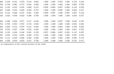
The results of the power of the tests are presented in Table 2. There are several features that are noteworthy. First, the power is generally good and increases steadily asT grows. However, the power is not necessarily increasing in N. In particular, the power of the individually computed tests displays no tendency of increasing as N grows. Of course, this casts doubts on the argument that pooling the data in the way suggested by Mark and Sul (2001) should generate more powerful tests.
Second, there is generally no advantage to pooled LSDV estimation of the slope parameters in the forecasting equation. In fact, the power of the tests based on heterogenous LS estimated slopes can at times be higher than for those based on pooled slopes, especially whenT = 100, which is often satisfied in applied work. Of course, this result further reinforces the evidence against the claim that pooled estimation of the forecasting equation should generate more power.
Third, the power of the tests falls markedly as k grows. In fact, it is not unusual for the power to fall by as much as 50% when k increases from one to 10. This effect becomes even more pronounced as β departs from its hypothesized value of zero. For example, whenβ = 1, the results suggest that the power can fall by nearly 90% in some cases as k goes from one to 10. Hence, one explanation for the inability of the monetary model to outperform the random walk forecast could be that the tests are not powerful enough to detect it.
Fourth, the power can typically be increased significantly by pooling the individual test statistics. Because this effect is particularly pronounced when
the predictive ability of the monetary model, especially at longer horizons. The overall best power is obtained when using the Ssum statistic, which is
not unexpected given the homogenous alternative hypothesis considered in the simulations. In fact, the results suggest that the power of this test is effectively one in almost all experiments considered.
In summary, the Monte Carlo evidence provided in this section suggests that the power argument to pooling only the parameters of the forecasting equation is overstated and that it might be better to pool also the individual Diebold and Mariano (1995) statistics. The implication is that the inability of the monetary model to beat the random walk in previous work can be attributed in part to insufficient power.
6
Empirical results
This section reevaluates the empirical results of Mark and Sul (2001). The aim is to examine to what extent these hinge on pooling. Based on the results presented in the previous section, we hypothesize that pooling the parameters of the forecasting equation should not result in more frequent rejections of the equal predictability null.
As Rapach and Wohar (2004), we use the same data set used by Mark and Sul (2001). It comprises quarterly observation on nominal money supply, industrial production and nominal US dollar denominated exchange rates for 19 countries between 1973:Q1 and 1997:Q1. The data is mostly taken from the International Financial Statistics database of International Monetary Fund. For more details on the data, we make reference to Mark and Sul (2001).
Since the purpose is to reevaluate the forecasting results of Mark and Sul (2001), we will take their cointegration and homogeneity restrictions at face value. In fact, Rapach and Wohar (2004) examine the validity of these conditions and find that they appear to be quite realistic. Thus, the error coming from making the analysis conditional upon these restrictions should be relatively small.5
As in Mark and Sul (2001), we generate out-of-sample forecasts at two horizons, k = 1 and k = 16. In the case of pooled estimation, we initiate the forecasting recursion by fitting (4) using the LSDV estimator on the ob-servations available up until 1983:Q1 whereas, in the case of heterogenous estimation, the equation is fitted using LS. In either case, thek= 1 forecast-ing regression is used to forecast the exchange rate return in 1983:Q2 while
5
thek= 16 regression is used to forecast the exchange rate return in 1987:Q1. The sample is then updated by one period at the time and the forecasting procedure is repeated. This gives us 57 forecasts at the k= 1 horizon and 41 forecasts at thek= 16 horizon. These forecasts are then compared with those generated by the random walk model in (5).
To measure the relative forecast accuracy, we use both the individual and pooled bootstrap U and S statistics. As before, the null hypothesis is formu-lated so that the monetary and random walk models provide equally accurate forecasts in which caseU = 1 andS= 0. The null hypothesis is tested against the one-sided alternative that the forecast produced by the monetary model is more accurate than that produced by the random walk model. Thus, under the alternative hypothesis, we haveU <1 andS <0.
For convenience of comparison with the Mark and Sul (2001) results, we use seemingly unrelated regressions to estimate the bootstrap data generating process and we augment the forecasting equation with common time effects to account for at least some cross-sectional dependency. All results are based on 1,000 bootstrap replications. As in Mark and Sul (2001), the results for the individual test statistics are organized based on the choice of numeraire country. There are three such countries, US, Japan and Switzerland.
The forecasting results based on US as numeraire are presented in Table 3. Based on the S statistic, the null of equal forecasting accuracy cannot be rejected at any conventional significance level for any of the countries. Thus, based on this statistic, there appears to be no advantage to pooled LSDV estimation of the forecast equation. The results for the U statistic are quite different. At the k = 1 horizon, we see that, while the equal forecast null cannot be rejected for any of the countries on the 10% level for the LS based forecasts, it is rejected eight times for the LSDV forecasts. At the k = 16 horizon, the null is rejected on 15 occasions for the LSDV based forecasts and on six occasions for the LS based ones. Thus, based on the U statistic, we actually do end up rejecting the null more frequently when pooling the parameters of the forecasting equation.
Table 4 contains the results with Japan as numeraire. In this case, the equal forecast null can be rejected on two occasions on the 10% level when using the S statistic, for Austria and Italy at the k= 16 horizon. As in the US case, the results for the U statistic are more significant. When k= 1, the null is rejected three times with all rejections being for the LSDV forecasts. Whenk= 16, the null is rejected four times for the LSDV based forecasts and three times for the LS based ones. Thus, in this case, there is little evidence to suggest that the tests based on LSDV estimation should be more powerful than those based on LS estimation.
based on the LS forecasts. All seven rejections occur at the k = 16 horizon. Moreover, at the k = 1 horizon, the U statistic leads to 16 rejections for the LSDV based forecasts and to four rejections for the LS based ones. At the
k= 16 horizon, we count 14 rejections for the LSDV forecasts and 10 rejections for the LS forecasts. Hence, as in the US case, we find some evidence that pooling the forecasting equation can lead to more powerful tests.
The results of the Diebold and Mariano (1995) statistic reported so far seem to provide no evidence of predictability. However, as illustrated in Sec-tion 5, the fact that rejecting the equal predictability null is difficult need not reflect the actual data but rather the low power of the test itself. If this is the case, then pooling the individual test statistics should lead to augmented power.
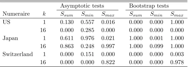
The results on the pooled statistics are reported in Table 6. We see that the null can be safely rejected on all conventional significance levels for US and Switzerland when using the bootstrap Ssum and Smin statistics. For
the Smin statistic, the null is also rejected on the 10% level for Japan. The
interpretation is that the null can be rejected for all countries when using US and Switzerland as numeraire countries, and that it can be rejected for at least one country when using Japan as numeraire, which corroborate our earlier findings based on the U statistic.6 The results for Smax are less encouraging,
which is not unexpected given the results presented in Section 5 suggesting that the power of this test can sometimes be quite poor. Moreover, although somewhat less significant, we see that the results for the asymptotic tests generally corroborate those for the bootstrapped ones.
To summarize, the results presented in this section provide little evidence to support the argument that pooled estimation of the forecast equation should lead to more powerful tests. Of course, this finding is well in line with the Monte Carlo evidence provided in Section 5, and so are the relative rejec-tion frequency between the S and U statistics. Consistent with the Monte Carlo results, we find that the evidence of predictability becomes clearer when pooling the individual test statistics. Thus, unlike Mark and Sul (2001), who report only weak evidence in favor of the monetary model, our results are more encouraging, which is interesting in view of the recent research that purport
6
to shed light on exchange rate predictability by exploiting recent advances in panel data econometrics.
7
Conclusions
The difficulty in predicting future exchange rate movements based on the mon-etary model has been a longstanding problem in the international economics literature. One explanation as to why the monetary model seem to be unable to beat the simple random walk forecast is that conventionally applied time series tests may not be powerful enough to reject the null of equal forecast accuracy, especially considering the short time span of the data available on the post Bretton Woods float. If this is the case, then the use of larger panel data sets should be able to generate more powerful tests. However, for an explanation so commonly held, it is surprising that there is so little evidence to support it.
This paper undertakes an extensive evaluation of the power argument to panel data tests of forecast accuracy. This is accomplished by first providing Monte Carlo evidence on the power properties of several pooled versions of the Theil U statistic and the S prediction statistics of Diebold and Mariano (1995). These findings are then illustrated through an empirical application. Two types of pooling are considered. The first is that of Mark and Sul (2001) and involves pooling only the parameters of the forecasting equation. The second is to pool not only the forecasting parameters but also the individual prediction statistics.
The Monte Carlo evidence suggests that, while pooled estimation of the forecasting equation does not lead to any gains in power, pooling the indi-vidual test statistics usually results in large gains in power, especially at long forecast horizons. This suggests that the inability of the monetary model to outperform the random walk in forecast competitions may be attributed in part to insufficient power. In the empirical part of the paper, the data set of Mark and Sul (2001) is employed. It is shown that pooling the individual tests results in more evidence in favor of the monetary model.
instability, there is a possibility that there are breaks in the data that we have not accounted for. Again, the results of Rapach and Wohar (2004) indicate that this is not the case. Yet another limitation is the assumed presence of cointegration but, as pointed out earlier, this restrictions has also been shown to hold.7
7
References
Banerjee, A., Marcellino, M., and Osbat, C. (2004). Some cautions on the use of panel methods for integrated series of macroeconomic data. Econo-metric Journal 7, 322-340.
Banerjee, A., Marcellino, M., and Osbat, C. (2005). Testing for PPP: Should we use panel methods? Empirical Economics 30, 77-91.
Berben, R.-P., and van Dijk, D. J. C. (1998). Does the absence of cointegra-tion explain the typical findings in long horizon regressions? Economet-ric Institute Report 145, Erasmus University Rotterdam, EconometEconomet-ric Institute.
Berkowitz, J., and Giorgianni, L. (2001). Long-horizon exchange rate pre-dictability? Review of Economics and Statistics 83, 81-91.
Diebold, F. X., and Mariano, R. S. (1995). Comparing predictive accuracy.
Journal of Business and Economic Statistics 13, 253-63.
Engel, C. (2000). Long-run PPP may not hold after all. Journal of Interna-tional Economics 51, 243-73.
Gengenbach, C., Palm, F. C., and Urbain, J-P. (2006). Panel cointegration testing in the presence of common factors. Oxford Bulletin of Economics and Statistics 68, 683-719.
Groen, J. J. J. (1999). Long-horizon predictability of exchange rates: Is it for real? Empirical Economics 24, 451-69.
Groen, J. J. J. (2000). The monetary exchange rate model as a long-run phenomenon. Journal of International Economics 52, 299-319.
Kilian, L. (1999). Exchange rates and monetary fundamentals: What do we learn from long-horizon regressions? Journal of Applied Econometrics
14, 491-510.
Mark, N. C. (1995). Exchange rates and fundamentals: Evidence on long-horizon predictability. American Economic Review 85, 201-18.
Mark, N. C., and Sul, D. (2001). Nominal exchange rates and monetary fun-damentals: Evidence from a small post-Bretton Woods panel. Journal of International Economics 53, 29-52.
Meese, R. A., and Rogoff, K. (1983). Empirical exchange rate models of the seventies: Do they fit out of sample? Journal of International Economics
Papell, D. H. and Theodoridis, H. (2001). The choice of numeraire currency in panel tests of purchasing power parity. Journal of Money, Credit and Banking 33, 790-803.
Rapach, D. E., and Wohar, M. E. (2002). Testing the monetary model of exchange rate determination: New evidence from a century of data.
Journal of International Economics 58, 359-385.
Rapach, D. E., and Wohar, M. E. (2004). Testing the monetary model of exchange rate determination: A closer look at panels. Journal of Inter-national Money and Finance 23, 867-895.
Taylor, M. P., and Sarno, L. (1998). The behavior of real exchange rates dur-ing the post-Bretton Woods period. Journal of International Economics
Table 1: Size at the 5% level.
Individual statistics Pooled statistics
k T N Slsdv S
a lsdv U
a
lsdv Sls S
a
ls U
a
ls Ssum S
a
sum Smin S
a
min Smax S
a max
ρ= 0b
1 50 10 0.040 0.039 0.055 0.006 0.013 0.025 0.000 0.010 0.050 0.130 0.000 0.040 1 100 10 0.035 0.040 0.072 0.003 0.017 0.027 0.000 0.010 0.020 0.187 0.007 0.047 1 50 20 0.045 0.043 0.071 0.008 0.018 0.026 0.003 0.010 0.047 0.240 0.007 0.107 1 100 20 0.041 0.042 0.067 0.005 0.014 0.024 0.007 0.027 0.030 0.227 0.010 0.160 10 50 10 0.213 0.015 0.020 0.140 0.010 0.028 0.170 0.000 0.747 0.030 0.000 0.070 10 100 10 0.143 0.017 0.026 0.064 0.007 0.050 0.100 0.003 0.427 0.047 0.003 0.043 10 50 20 0.255 0.013 0.012 0.142 0.010 0.034 0.217 0.000 0.917 0.010 0.000 0.100 10 100 20 0.156 0.019 0.015 0.059 0.007 0.046 0.153 0.003 0.607 0.053 0.003 0.110
ρ= 1c
1 50 10 0.036 0.037 0.066 0.007 0.019 0.028 0.010 0.023 0.050 0.153 0.010 0.047 1 100 10 0.031 0.037 0.068 0.006 0.014 0.024 0.003 0.017 0.013 0.193 0.007 0.023 1 50 20 0.043 0.043 0.065 0.007 0.021 0.025 0.003 0.007 0.033 0.263 0.013 0.097 1 100 20 0.037 0.042 0.066 0.007 0.017 0.029 0.007 0.023 0.043 0.233 0.013 0.103 10 50 10 0.243 0.017 0.021 0.149 0.009 0.034 0.220 0.003 0.757 0.047 0.007 0.093 10 100 10 0.134 0.015 0.024 0.062 0.011 0.052 0.087 0.007 0.387 0.090 0.003 0.067 10 50 20 0.247 0.016 0.012 0.145 0.014 0.034 0.200 0.000 0.913 0.013 0.000 0.107 10 100 20 0.160 0.016 0.016 0.059 0.007 0.050 0.143 0.003 0.607 0.077 0.000 0.107
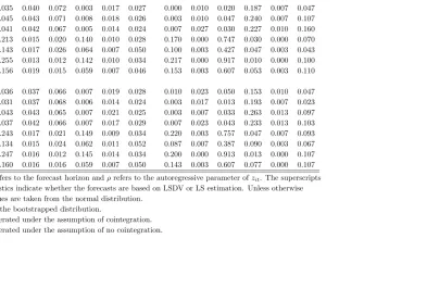
Notes: The value krefers to the forecast horizon andρrefers to the autoregressive parameter ofzit. The superscripts of the individual statistics indicate whether the forecasts are based on LSDV or LS estimation. Unless otherwise stated the critical values are taken from the normal distribution.
a
The test is based on the bootstrapped distribution. b
The bootstrap is generated under the assumption of cointegration.
Table 2: Raw power at the 5% level.
Individual statistics Pooled statistics
k T N Slsdv S
a lsdv U
a
lsdv Sls S
a
ls U
a
ls Ssum S
a
sum Smin S
a
min Smax S
a max
ρ= 0b
1 50 10 0.458 0.432 0.839 0.370 0.438 0.673 1.000 1.000 0.867 1.000 0.737 0.510 1 100 10 0.798 0.759 0.967 0.775 0.804 0.946 1.000 1.000 1.000 1.000 0.957 0.873 1 50 20 0.469 0.433 0.841 0.379 0.444 0.662 1.000 1.000 0.953 1.000 0.740 0.243 1 100 20 0.780 0.746 0.965 0.757 0.804 0.936 1.000 1.000 1.000 1.000 0.963 0.790 10 50 10 0.534 0.128 0.352 0.359 0.086 0.215 0.950 0.963 0.987 0.993 0.133 0.233 10 100 10 0.667 0.336 0.858 0.628 0.322 0.781 1.000 1.000 0.993 1.000 0.623 0.547 10 50 20 0.543 0.142 0.366 0.357 0.081 0.203 0.993 0.997 1.000 0.997 0.097 0.150 10 100 20 0.656 0.322 0.840 0.622 0.306 0.769 1.000 1.000 1.000 1.000 0.500 0.357
ρ= 1c
1 50 10 0.464 0.400 0.804 0.371 0.417 0.648 1.000 1.000 0.897 1.000 0.643 0.423 1 100 10 0.784 0.708 0.955 0.767 0.782 0.926 1.000 1.000 1.000 1.000 0.933 0.880 1 50 20 0.462 0.388 0.812 0.370 0.412 0.646 1.000 1.000 0.963 1.000 0.700 0.263 1 100 20 0.783 0.702 0.957 0.766 0.782 0.928 1.000 1.000 1.000 1.000 0.957 0.793 10 50 10 0.539 0.150 0.338 0.348 0.085 0.193 0.957 0.960 0.987 0.983 0.147 0.297 10 100 10 0.667 0.322 0.852 0.635 0.306 0.785 1.000 1.000 1.000 1.000 0.597 0.523 10 50 20 0.549 0.144 0.359 0.360 0.083 0.200 1.000 1.000 1.000 1.000 0.083 0.170 10 100 20 0.664 0.329 0.858 0.633 0.315 0.786 1.000 1.000 1.000 1.000 0.553 0.417
Notes: See Table 1 for an explanation of the various features of the table.
Table 3: Forecasts with US as numeraire country.
k= 1 k= 16
LSDV LS LSDV LS
Country S p-val U p-val S p-val U p-val S p-val U p-val S p-val U p-val
UK −0.58 0.63 0.98 0.08 −0.22 0.52 0.99 0.28 −1.14 0.27 0.57 0.00 −0.31 0.39 0.95 0.29
Austria −0.70 0.78 0.98 0.04 −0.59 0.50 0.99 0.49 −0.67 0.39 0.84 0.06 −1.13 0.23 0.83 0.11
Belgium −0.05 0.86 1.00 0.75 −0.56 0.61 0.99 0.57 −1.43 0.22 0.41 0.00 1.28 0.67 1.26 0.84
Denmark 0.52 0.91 1.01 1.00 1.71 0.90 1.00 0.80 −0.41 0.40 0.86 0.07 0.08 0.46 1.02 0.50
France −0.27 0.95 0.99 0.40 −0.91 0.64 0.99 0.14 −1.29 0.25 0.58 0.00 1.17 0.71 1.06 0.70
Germany −0.52 0.95 0.99 0.05 0.83 0.50 1.06 1.00 −1.28 0.27 0.52 0.00 −0.76 0.38 0.71 0.00
Netherland −0.64 0.83 0.99 0.06 −0.47 0.49 0.99 0.50 −1.02 0.32 0.70 0.00 −1.13 0.28 0.76 0.04
Canada −0.36 0.53 0.99 0.08 1.61 0.71 1.04 0.51 −2.09 0.13 0.55 0.00 −0.57 0.26 0.83 0.15
Japan 0.08 0.96 1.00 1.00 −0.45 0.45 0.99 0.23 −0.02 0.51 1.00 0.50 −0.37 0.45 0.92 0.22
Finland 0.04 0.77 1.00 0.83 0.65 0.73 1.02 0.96 −0.72 0.35 0.86 0.09 −1.07 0.28 0.86 0.13
Greece 0.86 0.89 1.02 0.99 2.82 0.94 1.22 1.00 0.17 0.50 1.05 0.63 3.58 0.95 1.53 0.99
Spain −0.12 0.88 1.00 0.52 0.72 0.79 1.04 0.84 −1.11 0.26 0.67 0.00 −0.50 0.41 0.82 0.06
Australia 0.85 0.97 1.02 1.00 2.92 0.30 1.22 0.23 −0.41 0.41 0.86 0.10 1.61 0.66 1.52 0.81
Italy −0.12 0.83 1.00 0.54 0.42 0.74 1.01 0.93 −1.10 0.29 0.75 0.01 −1.04 0.31 0.85 0.05 Switzerland −0.92 0.83 0.98 0.03 0.07 0.67 1.00 0.68 −1.98 0.18 0.75 0.01 −1.12 0.26 0.83 0.06
Korea −1.70 0.27 0.91 0.01 0.85 0.45 1.09 0.73 −1.79 0.14 0.49 0.00 −1.77 0.14 0.66 0.03
Norway −0.07 0.81 1.00 0.68 0.68 0.72 1.01 0.84 −1.64 0.22 0.54 0.00 −0.08 0.50 0.99 0.47 Sweden −1.08 0.61 0.98 0.02 0.42 0.78 1.01 0.83 −1.61 0.20 0.37 0.00 −2.16 0.11 0.87 0.16
Notes: The out-of-sample forecasts for the monetary model are compared to those for the random walk model. Thep-values are computed as the
Table 4: Forecasts with Japan as numeraire country.
k= 1 k= 16
LSDV LS LSDV LS
Country S p-val U p-val S p-val U p-val S p-val U p-val S p-val U p-val
US 0.22 1.00 1.01 1.00 0.67 0.60 1.03 1.00 0.29 0.57 1.08 0.76 1.47 0.78 1.80 1.00
UK 0.84 0.92 1.05 1.00 1.51 0.86 1.06 1.00 3.59 0.96 2.09 1.00 4.53 0.98 2.28 1.00
Austria −0.13 0.86 1.00 0.68 −0.25 0.40 0.99 0.41 −0.46 0.48 0.95 0.34 −3.57 0.03 0.86 0.17
Belgium 0.90 0.96 1.04 1.00 −0.13 0.67 1.00 0.65 1.43 0.82 1.55 1.00 1.45 0.76 2.81 1.00
Denmark −0.13 0.75 1.00 0.49 −0.16 0.55 1.00 0.55 −0.65 0.42 0.83 0.07 −0.20 0.46 0.95 0.34
France 0.14 0.99 1.01 1.00 0.23 0.67 1.01 0.97 −0.09 0.51 0.97 0.43 −0.32 0.48 0.93 0.23
Germany 0.24 1.00 1.01 1.00 1.70 0.58 1.11 1.00 1.83 0.89 1.34 0.98 3.98 0.98 1.91 1.00
Netherland 0.02 0.94 1.00 0.96 0.00 0.50 1.00 0.50 0.00 0.57 1.00 0.57 −1.33 0.19 0.85 0.14
Canada 0.42 0.99 1.02 1.00 0.37 0.77 1.01 0.73 −0.42 0.42 0.91 0.19 0.00 0.47 1.00 0.47
Finland −0.65 0.67 0.98 0.03 −0.53 0.52 0.98 0.11 −2.15 0.13 0.66 0.00 −1.89 0.16 0.86 0.12
Greece −0.26 0.69 0.99 0.34 3.82 0.99 1.42 1.00 −0.50 0.46 0.91 0.24 −1.15 0.33 0.88 0.18
Spain −0.89 0.87 0.98 0.00 −0.10 0.75 1.00 0.72 −1.89 0.17 0.56 0.00 −1.72 0.20 0.54 0.00
Australia −0.15 0.94 1.00 0.62 1.00 0.48 1.09 0.53 −0.26 0.44 0.96 0.34 3.00 0.91 1.72 0.98
Italy −0.51 0.87 0.98 0.01 −1.02 0.57 0.98 0.17 −1.24 0.27 0.77 0.03 −2.74 0.08 0.78 0.02
Switzerland 0.20 0.95 1.01 0.99 0.82 0.68 1.05 0.70 0.20 0.59 1.02 0.61 0.40 0.45 1.05 0.47 Korea −0.30 0.90 0.99 0.13 1.07 0.88 1.09 0.99 −0.30 0.47 0.91 0.22 −1.18 0.25 0.67 0.03
Norway 0.80 0.95 1.04 1.00 0.85 0.74 1.01 0.93 2.76 0.94 1.77 1.00 1.59 0.81 1.26 0.93
Sweden 0.44 0.96 1.02 1.00 1.41 0.96 1.05 0.99 2.50 0.92 1.57 1.00 0.00 0.46 1.00 0.46
Notes: See Table 3 for an explanation of the various features of the table.
Table 5: Forecasts with Switzerland as numeraire country.
k= 1 k= 16
LSDV LS LSDV LS
Country S p-val U p-val S p-val U p-val S p-val U p-val S p-val U p-val
US −0.98 0.79 0.98 0.01 −0.60 0.48 0.99 0.09 −1.54 0.20 0.78 0.02 1.24 0.71 1.37 0.98
UK −0.96 0.84 0.97 0.00 −0.18 0.59 0.99 0.30 2.32 0.90 1.47 1.00 2.85 0.93 1.89 1.00
Austria −1.52 0.72 0.98 0.00 −1.45 0.70 0.98 0.54 −2.30 0.18 0.65 0.00 −2.32 0.15 0.75 0.01
Belgium −1.00 0.86 0.95 0.00 −0.24 0.84 1.00 0.73 −2.13 0.16 0.65 0.00 1.19 0.72 2.16 1.00 Denmark −1.42 0.63 0.96 0.00 1.00 0.77 1.01 0.87 −1.77 0.19 0.70 0.00 −1.71 0.19 0.84 0.07
France −2.36 0.15 0.92 0.00 −2.10 0.18 0.94 0.00 −4.68 0.02 0.32 0.00 −3.50 0.04 0.64 0.00
Germany −0.76 0.68 0.98 0.00 1.18 0.69 1.11 1.00 −2.84 0.12 0.49 0.00 0.49 0.67 1.12 0.86
Netherland −2.05 0.60 0.96 0.00 −1.87 0.35 0.94 0.68 −2.90 0.11 0.38 0.00 −2.80 0.07 0.53 0.00
Canada −0.35 0.94 1.00 0.36 0.48 1.00 1.01 1.00 −1.78 0.17 0.59 0.00 −1.03 0.27 0.81 0.03
Japan 0.15 0.91 1.00 0.99 0.88 0.57 1.01 0.81 0.07 0.56 1.01 0.57 −1.20 0.30 0.91 0.25
Finland −2.03 0.62 0.96 0.00 −2.76 0.21 0.95 0.00 −3.22 0.05 0.70 0.00 −2.76 0.07 0.88 0.12
Greece −1.01 0.84 0.99 0.02 1.82 0.43 1.16 1.00 −0.61 0.45 0.85 0.09 −1.07 0.35 0.77 0.05
Spain −1.66 0.85 0.96 0.00 −1.12 0.92 0.95 0.72 −2.18 0.13 0.48 0.00 −1.74 0.16 0.48 0.00
Australia −0.90 0.93 0.99 0.01 0.06 0.99 1.00 0.99 −0.86 0.32 0.80 0.02 1.85 0.85 1.43 0.98
Italy −1.79 0.10 0.97 0.00 −1.49 0.14 0.98 0.04 −2.71 0.09 0.58 0.00 −2.77 0.08 0.74 0.02
Korea −1.27 0.90 0.98 0.00 −0.51 0.82 0.98 0.48 −2.07 0.17 0.38 0.00 −2.10 0.15 0.40 0.00
Norway −1.29 0.81 0.95 0.00 −0.04 0.62 1.00 0.60 0.79 0.65 1.38 0.98 2.73 0.92 1.50 0.99
Sweden −1.33 0.87 0.95 0.00 −0.91 0.85 0.96 0.23 −0.21 0.47 0.95 0.33 −1.57 0.23 0.62 0.00
Notes: See Table 3 for an explanation of the various features of the table.
Table 6: Pooled predictability tests.
Asymptotic tests Bootstrap tests
Numeraire k Ssum Smin Smax Ssum Smin Smax
US 1 0.130 0.557 0.016 0.000 0.000 1.000 16 0.000 0.285 0.000 0.000 0.000 0.000 Japan 1 0.611 0.976 0.021 1.000 0.001 1.000 16 0.863 0.248 0.997 1.000 0.099 1.000 Switzerland 1 0.000 0.151 0.000 0.000 0.000 0.003 16 0.000 0.000 0.822 0.000 0.000 0.978