Munich Personal RePEc Archive
Testing for breaks in cointegrated panels
Di Iorio, Francesca and Fachin, Stefano
July 2006
Online at
https://mpra.ub.uni-muenchen.de/3280/
Testing for breaks in cointegrated panels
Francesca Di Iorio Stefano Fachin
University of Naples Federico II University of Rome ”La Sapienza”
Abstract
Stability tests for cointegrating coefficients are known to have very low power with small to medium sample sizes. In this paper we propose to solve this problem by extending the tests to dependent cointegrated pan-els through the stationary bootstrap. Simulation evidence shows that the proposed panel tests improve considerably on asymptotic tests applied to individual series. As an empirical illustration we examined investment and saving for a panel of 14 European countries over the 1960-2002 period. While the individual stability tests, contrary to expectations and graphical evi-dence, in almost all cases do not reject the null of stability, the bootstrap panel tests lead to the more plausible conclusion that the long-run relation-ship between these two variables is likely to have undergone a break.
Keywords: Panel cointegration, stationary bootstrap, parameter stabil-ity tests, FM-OLS.
JEL codes: C23, C15
1
Introduction
1The analysis of cointegration in non-stationary panels has been recently rapidly expanding in two main directions. Thefirst, urged by the nature of the data actually used in empirical applications, is the effort to generalise the tests to the case of dependent units, either by modelling the dependence (inter alia, Gengenbach, Palm, Urbain, 2005) or reproducing it through the bootstrap (Fachin, 2006, Westerlund and Edgerton, 2006). The second direction follows steps already taken by the cointegration literature in the early ’90’s, tackling the issues of testing (i) cointegration allowing for breaks and (ii) the stability of a cointegrating relationship. In this stream of the literature, the first problem seems to have received more attention (e.g., Banerjee and Carrion-i-Silvestre, 2004 and 2006, Gutierrez, 2005, Wester-lund, 2006) than the second (to the best of our knowledge, only Emerson and Kao, 2001, 2005, for trend regressions, Kao and Chiang, 2000, for ho-mogenous panel regressions). This is somehow surprising, as stability tests with unknown break points may have very low power with even medium sample sizes. For instance, the rejection rates underH1 simulated by
Gre-gory, Nason and Watt (1996) forT = 100 and medium speed of adjustment are only marginally higher than Type I errors, and actuallylower than the significance level. Cointegration stability tests are thus natural candidates for panel extensions hopefully able to grant power gains large enough to make them empirically useful. A second surprising aspect of the current de-bate is that so far the developments in the treatment of dependence across units seems to have been largely ignored in the ”panel with breaks” liter-ature2. The tests proposed should thus be regarded essentially as a first
step in the construction of empirically relevant procedures, very much like thefirst generation panel cointegration tests. On the contrary, in this paper we tackle the dependence issue from the outset, proposing a panel general-isation of Hansen (1992) stability tests based on the stationary bootstrap
1
Financial support from the Department of Statistics of the University of Naples Fed-erico II, University of Rome ”La Sapienza” and MIUR is gratefully acknowledged. We are grateful to Anindya Banerjee and Josep Carrion-i-Silvestre for kindly providing the invest-ment and savings data set and to participants to the SIS Turin and Cambridge Panel Data 2006 conferences for suggestion and comments. Correspondence to: [email protected], [email protected].
2
Noticeable exceptions include the panel cointegration tests with breaks by Banerjee and Carrion-i-Silvestre (2004, 2006) and Westerlund (2006), which however leave many questions open. Westerlund applies simple resampling to data which, provided cointegra-tion holds, are weakly dependent, while Banerjee and Carrion-i-Silvestre’s (2004) proce-dure impliesfitting an AR model to a MA process with a unit root under no cointegration (the same remark applies to Westerlund and Edgerton, 2006). Finally, Banerjee and Carrion-i-Silvestre (2006) test appears to have very good properties, but since it is based on Bai and Ng’s (2004) PANIC procedure it unfortunately requires rather large sam-ple sizes (the smallest ones reported in Banerjee and Carrion-i-Silvestre’s simulations are
which is completely robust to cross-section dependence, and may thus be helpful for actual empirical work.
We shall now (section 2) introduce the set-up and outline the testing procedure, then present the design and results of a Monte Carlo experiment (section 3) and an empirical illustration on the stability of the relation-ship between the investment/GDP and savings/GDP ratios, the so-called Feldstein-Horioka puzzle (section 4). Some conclusions and suggestions for future research arefinally discussed (section 5).
2
Testing parameter stability in cointegrated
pan-els
2.1
Set-up
Consider a (k+ 1)−dimensional I(1) random variable Z observed over N units and T time periods (respectively indexed by i and t), naturally par-titioned asZit = [YitX1it. . . Xkit]0, with cointegration assumed to hold
be-tween Yit and X0it = [X1it. . . Xkit]0. Then, as long as no long-run
relation-ships among the X0s exist, we can estimate the N cointegrating vectors
(say, βi = [βi1βi2. . .βik]) by applying some single-equation method (e.g. FM-OLS) separately to each of the N time series. Hansen (1992) proposed three tests for the hypothesis that the β’s are stable over time when no a priori information on the location of the possible breaks tb
i is available:
(i) the maximum of the Chow tests computed at all possible break points (SupF); (ii) their mean (M eanF); (iii) a Lagrange-Multiplier test of the hypothesis that the coefficients follow a martingale process of zero variance (Lc). The panel extension along the lines of Pedroni’s (1999) group mean
test is in principle trivial, as it involves simply taking the mean (or some robust statistic such as the median or anα−trimmed mean) of the statistics computed for the individual units. Similarly to the case of panel cointe-gration tests, the bootstrap is a natural candidate for solving the problem of inference under the general set-up of dependent units. To this end, we need to design a resampling scheme delivering pseudodata obeying the null hypothesis of coefficient stability and reproducing both the autocorrelation and cross-correlation properties of the data. Denoting by Si the stability
statistic of interest for unit i, we propose to estimate the p−value of the group stability statisticS by the following algorithm:
1. Obtain estimatesβb0i of the cointegrating vectors underH0 : coefficient
stability;
2. Compute the individual stability statistics Sbi and estimate break
3. Compute the group stability statisticS,b e.g.,Sbm=PNi=1Sbi/N, orSbme
=median(Sb), where Sb=hSb1, . . . ,SbNi;
4. Estimate models allowing for breaks at the periods etb
i and store the
residuals bet = [be1t. . .beN t] ; the choice of the etb0
i s, a key point of the
procedure, is discussed in some detail in Remark (i) below;
5. Since cointegration holds, in resampling theT×NmatrixEb = [be1. . .beT]0 we only need to allow for short-run autocorrelation. Hence, we can ap-ply the stationary bootstrap (Politis and Romano, 1994) and obtain a matrix of pseudo-residuals E∗ = [e∗
1. . .e∗T]0 reproducing both the
short-run correlation over time and the cross-units correlation of the estimated residuals;
6. Construct the pseudodata Yit∗ under H0 : coefficient stability by
ap-pendinge∗it toβb0iX0
it;
7. Compute the group stability statisticS∗for the pseudo-data set [Yit∗X0
it]0 , i=
1, . . . , N, t= 1, . . . , T;
8. Repeat steps (5)-(7) a large number (say,B) of times;
9. Compute the boostrap estimate of thep−value asp∗ =prop(S∗ >S).b
Three remarks are in order:
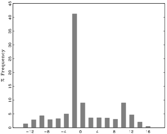
(i) As mentioned above, estimation of break points is a key point of the procedure. An apparently appealing choice is btb
i = arg max(SupFbi),
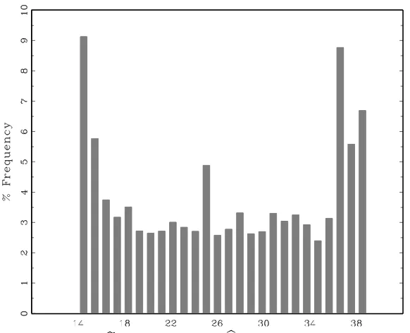
so that break location is allowed to vary across units. In fact, this is a good choice when there is a break in the data (for instance, in the simulation reported in Fig. 1 the mean estimation error is 0.73 and the median error 1), but not so much so whenH0: no break holds. In these
circumstances in small time samples the break is often placed towards either end of the sample (see Fig. 2), causing overfitting and spuriously small estimated residuals. As a consequence of the latter, the boot-strap pseudodata tend to exhibit spuriously high signal/noise ratios, and the bootstrap stability tests to be severely oversized. Superior results are obtained when the restriction of a common break located at the median of the individual estimates of break periods is imposed (i.e., etb
i = median(btb), btb =
£b
tb
1btb2. . .btbN
¤
, and btb
i = arg max(SupFbi)
∀i).
(iii) Although exploratory simulations showed the results to be quite robust to the choice of block length, in principle this is a critical point of the algorithm. Here for computational convenience we applied a simple rule-of-thumb,fixing it atT /10. In future work we plan to implement Politis and White’s (2003) algorithm.
Fig. 1. Distribution of the error in the estimation of the breakpoint
b
tb
i −tbi,wherebtbi = arg max(SupFbi) and tbi ∼U nif orm[0.5T −3,0.5T+ 3]
Fig. 2. Distribution ofbtb
i = arg max(SupFbi), T = 50,25% trimming at each
sample end, when there is no break in the cointegrating coefficients. Pooled results from 500 Montecarlo replications for 40 units.
3
Monte Carlo Experiment
3.1
Design
The simulation experiment is based on the design adopted by Fachin (2006), essentially a generalisation of the Engle and Granger (1987) classical Data Generation Process (DGP) to the case of dependent panels (a similar design in also employed bye.g. Kao, 1999). Considering for the sake of simplicity the bivariate case Zit= [YitXit]0 the DGP can be summarised as follows.
Following Pesaran (2006), short-run dependence is induced by defining the shocks driving Y and X (uj, j = x, y) as the sum of a idiosyncratic
com-ponent (²j, j = x, y) and a single stationary common factor (fj
t, j = x, y);
long-run dependence is caused by an explanatory variable common across units. Lettingtb be the period in which the break takes place, we then have:
xit = (1−a1)−1a1uyit+u x
it (1)
yit =
½
μ0i+β0xit+uyit, t≤tbi
μ1i+β1xit+uyit, t > tbi
(2)
are generated as:
½
ux
it=γxiftx+²xit
uyit=γyifty+²yit . (3)
The coefficientsγji, j = x, y, are the factor loadings and determine the strength of the short-run cross-correlation across units; hereγji ∼U nif orm(−1,6) ∀i, j,so that the cross-correlation is substantial (about 0.65). The structure of the idiosyncratic component is:
½
²x
it=
Pt
j=1(exit−j+θ)
²yit=φi²yit−1+eyit (4)
whereφi ∼U nif orm(0.2,0.4). Finally,
½
ex
it∼N(0,σ2ix)
eyit∼N(0,σ2iy) (5)
withσ2ij ∼U nif orm(0.5,1.5), j =x, y, so to allow for some heterogene-ity across units.
The DGP (1)-(5) is obviously quite complex. Rather than aiming at the unfeasible task of a complete design3 we will define as a base case an
empirically relevant set-up and then explore a few interesting variations. Considering that the simple bivariate DGP often used in simulation exper-iments is clearly unrealistic, but in single-equation cointegration modelling the number of explanatory variables is usually limited, we generally setk= 2 in both the DGP and estimated model. With no loss of generality we set both constant and slopes to 3 before the break (the same value chosen by Banerjee and Carrion- i-Silvestre, 2004, for the slope); after the break all co-efficients are halved. Finally,a1 = 0, so that theX variables are exogenous.
Since Gregory, Nason and Watt (1996) report a tendency to overrjection of the asymptotic test in models with 3 or 4 explanatory variables we also run a separate experiment with k = 4. Finally, a key point is that given the rather short time series analysed in most experiments, in order to ensure computational stability wefixed the trimming coefficient at 25%. The cases considered are six altogether.
1. Base case: T = 50, N from 5 to 40; in the power simulations break date Uniform over units in [0.5T ±3] = [22,28]. Since recursive sta-bility tests assume rather large sample sizes we chose tofix the time 3
sample in all experiments except the following one to 50. This is ad-mittedly a rather large sample in terms of annual data, but pretty small if a quarterly frequency is assumed. It may thus be considered relevant for actual empirical applications (note that it is much smaller than those typically considered in simulation studies on stability tests, where generallyT ≥100).
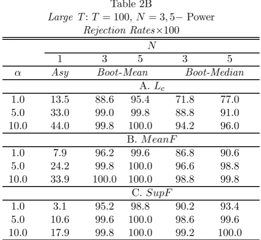
2. Large T: T = 100, N = 3,5; in the power simulations break date Uniform over units in [0.5T ±3]. Since the aim of this experiment is checking the time-asymptotic behaviour of the tests, for computational convenience only very small cross-section sample sizes are examined.
3. Late break: T = 50, N from 5 to 40; break date Uniform over units in [0.75T±3],that is [35,41].Since 25% of the sample is trimmed at each end, the estimation sample is [13,38]: the break can thus fall very close or even after the end of the estimation sample, a very demanding set-up.
The bootstrap algorithm described above is based on residuals of coin-tegrating regressions estimated for all units with a break at the median of the individual estimated break points, which is intuitively acceptable if we assume all units to be affected by breaks stemming from a common cause. However, even assuming each unit to be affected by at most one break over the period of interest, two rather different set-ups may arise: (i) the break periods may be widely disperse over units, for instance because they stem from different causes, each one relevant to only some units; (ii) some of the units may be not affected by a break at all. The two following cases are designed to investigate these two scenarios in turn:
4. Twin breaks: as Base case, but in half of the units the break date is Uniform in [0.3T±3] , and in the other half in [0.6T ±3].
5. Partial break: T = 50, N from 10 to 40, break date Uniform in [0.5T±3] over 0.7N units (the first seven in each block of ten), no break in the remaining units. This case deserves some discussion. The key question here is the following: what is the null hypothesis of the panel stability test (say,HP
0 )? LetH1i be that of the i−thindividual
test; then, one possibility is to take HP
0 = TNi H0i, so that the panel
null hypothesis is ”stability in all units”. However, this appears far too restrictive, especially in view of small sample applications where outliers may have an heavy influence on individual cases. Following Pedroni’s (2004) view of the meaning of panel cointegration tests, we prefer the panel null HP
0 : ”stability in a large number of units”. In
the cointegrating relationship is mostly, but not necessarily always, stable. As in the set-up of this experiment the answer is negative (H0
holds only in 30% of the units) we would like to have high rejection rates. Note that since this view of the test clearly requires fairly large cross-section sample sizes we setN ≥10.
6. Larger model: T = 50, N from 5 to 40, k = 4; break date Uniform over units in [0.5T ±3]. This case is designed exactly like the Base case, except the number of explanatory variables in both the DGP and estimated model.
To evaluate the improvements (in terms of both power gains and re-duction in size bias) which could be expected by moving from a standard time series to a panel set-up we also computed the average rejection rates of the asymptotic tests based on Hansen (1992) asymptotic critical values computed for all individual units involved in each experiment4. Note that
the comparison between the average performance of the asymptotic test on individual series and that of the panel tests with a smaller number of units (e.g., 5, 10 and 20 in the base case or 3 in the ”Large T” case) should be taken as merely suggestive of a pattern, as the units involved are not the same.
Finally, after some experimentation with different options we decided to
fix the number of Monte Carlo replications at 500 and that of bootstrap redrawings at 1000. Higher numbers of either would have delivered a small increase in the precision of the results not worth the large increase of the cost and time scale of the experiment (which, because of the recursive nature of the statistics evaluated, is computationally very demanding).
3.2
Results
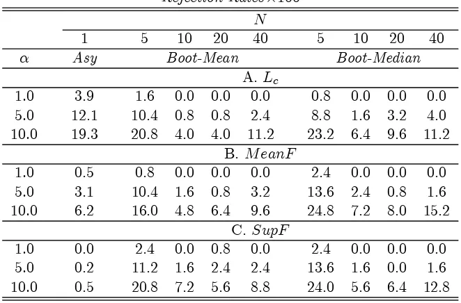
The results are reported in Tables 1A-6B below. In the Base case (T = 50, N from 5 to 40) the Type I errors (Table 1A) of the bootstrap panel tests have some positive size bias forN = 5 but converge fairly closely to nominal significance levels asN increases. The asymptotic tests on individual series deliver variable performances: the Lc test is slightly oversized, while both
theM eanF and the SupF appear to be conservative (more the latter than the former). The power gains offered by the panel tests are remarkable. Consistently witha prioriexpectations, the asymptotic tests have negligible power, while that of the panel tests is generally acceptable and definitely good forα= 10% andN ≥10 (e.g., 92% forN = 40, with Type I error 11%; Table 1B). Hence, using the panel tests grants considerable improvements
4
with respect to aggregate tests in terms of both reduction of size bias and increase in power. In fact, with this time sample a panel approach seems to be the only viable option. In comparative terms, we find the Type I errors to be very similar for all the three tests, while theSupF test appears to be somehow marginally less powerful than the Lc and M eanF. The
results of the mean and median panel tests also appear very similar. Since these findings hold approximately in all the cases examined the following comments are mostly expressed in general terms, with no reference to the specific tests.
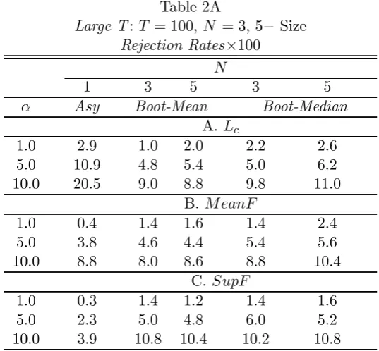
Allowing for the different speed of adjustment of the DGP’s employed, the ”LargeT” results (Tables 2A-2B) for the asymptotic tests are fully con-sistent with Gregory, Nason and Watt (1996): as we can see, the size bias is still noticeable, and power very poor. On the other hand, the Type I errors of the bootstrap panel tests essentially converge to nominal significance lev-els, and their power approaches 100% even with extremely smallN. Hence, even with a rather large time sample a panel approach seems preferable.
WhenT = 50 and breaks around 3/4 of the time sample (Table 3) power falls dramatically, rarely reaching 50% for the mean test; the performance of the median test, although not brilliant, appear somehow more robust. Since the upper extreme of the break interval (t= 41) falls after the end of the actual estimation sample (t= 38) thesefindings are not surprising, and make clear the great care necessary in using recursive stability tests.
The two experiments designed to check the robustness of the bootstrap procedure with respect to the nature of the breaks deliver comforting results. When the breaks come from two distributions, centred at the opposite ends of the sample (but not so close to them as in the previous case) the power loss caused by the misspecification of the cointegrating equation used to estimate the residuals to be bootstrapped is very small (Table 4). On the other hand, when 70% of the units are affected by the break it is interesting to see (Table 5) that the rejection rates seem to fall approximately in the same proportion (e.g., for N = 40 and α = 10% from 92.2% to 66.8%), so that if H0 does not hold in the majority of the units it is likely to be
rejected by the panel test as well. Somehow contrary to our expectations, in this set-up the mean and median tests deliver very similar results.
In a larger model with four explanatory variables (Tables 6A-B) we notice that the performance of the asymptotic tests is even worst than in the Base case. The Type I errors of the panel tests appear similar to the base case with only two variables, but unfortunately their power somehow smaller, possibly because the coefficient are estimated less precisely.
panel approach based on the bootstrap: in out experiments the Type I errors turned out to be generally close to nominal sizes and converging rather rapidly over both overT andN to nominal levels, and power from acceptable to good withα= 10% when the break is located around the middle of the sample. Although tests power does not appear to be much affected by a wide dispersion of the breaks across units and to be (correctly) roughly proportional to the fraction of breaking units, it is important to keep in mind that it can be disappointing if the breaks fall towards the end of the sample (which is not surprising, since with a small time sample the marginal information becomes very small).
Table 1A
Base Case: T = 50, N from 5 to 40 −Size
Rejection Rates×100 N
1 5 10 20 40 5 10 20 40 α Asy Boot-Mean Boot-Median
A. Lc
1.0 3.9 1.6 0.0 0.0 0.0 0.8 0.0 0.0 0.0 5.0 12.1 10.4 0.8 0.8 2.4 8.8 1.6 3.2 4.0 10.0 19.3 20.8 4.0 4.0 11.2 23.2 6.4 9.6 11.2
B. M eanF
1.0 0.5 0.8 0.0 0.0 0.0 2.4 0.0 0.0 0.0 5.0 3.1 10.4 1.6 0.8 3.2 13.6 2.4 0.8 1.6 10.0 6.2 16.0 4.8 6.4 9.6 24.8 7.2 8.0 15.2
C. SupF
1.0 0.0 2.4 0.0 0.8 0.0 2.4 0.0 0.0 0.0 5.0 0.2 11.2 1.6 2.4 2.4 13.6 1.6 0.0 1.6 10.0 0.5 20.8 7.2 5.6 8.8 24.0 5.6 6.4 12.8
DGP: No Break;
H0: No break;
Asy: average rejection rates of invidual tests over all 40 units, Hansen (1992) asymptotic critical values;
Boot-mean/median: bootstrap test on the mean/median across units of the stability statistics;
Bootstrap: 1000 redrawings, block sizeT /10;
Table 1B
Base Case: T = 50, N from 5 to 40−Power
Rejection Rates×100 N
1 5 10 20 40 5 10 20 40
α Asy Boot-Mean Boot-Median
A.Lc
1.0 3.5 6.6 5.6 6.4 5.2 7.4 10.6 11.6 10.0 5.0 11.5 36.4 39.8 55.0 59.4 41.0 44.4 55.0 58.6 10.0 19.3 57.0 73.2 87.6 92.2 62.0 70.2 77.6 84.8
B.M eanF
1.0 0.8 6.8 7.0 9.6 6.8 5.4 9.8 14.8 11.4 5.0 3.6 35.8 48.0 61.8 62.8 37.6 51.6 61.2 62.8 10.0 6.9 61.4 80.2 87.4 92.8 61.2 78.2 86.6 90.0
C. SupF
1.0 0.1 2.4 2.0 4.4 1.8 2.0 3.0 7.6 3.8 5.0 0.7 21.8 28.2 35.6 29.2 24.4 29.8 37.2 39.6 10.0 1.8 48.6 63.0 62.0 67.2 42.4 59.8 66.2 70.2
DGP: Break Uniform in [0.5T±3] = [22,28];
H0: No break;
Table 2A
Large T:T = 100, N = 3,5−Size
Rejection Rates×100 N
1 3 5 3 5
α Asy Boot-Mean Boot-Median
A. Lc
1.0 2.9 1.0 2.0 2.2 2.6 5.0 10.9 4.8 5.4 5.0 6.2 10.0 20.5 9.0 8.8 9.8 11.0
B. M eanF
1.0 0.4 1.4 1.6 1.4 2.4 5.0 3.8 4.6 4.4 5.4 5.6 10.0 8.8 8.0 8.6 8.8 10.4
C. SupF
1.0 0.3 1.4 1.2 1.4 1.6 5.0 2.3 5.0 4.8 6.0 5.2 10.0 3.9 10.8 10.4 10.2 10.8
DGP: No break;
H0: No break.
Asy: average rejection rates of invidual tests over all 5 units, Hansen (1992) asymptotic critical values;
Table 2B
Large T:T = 100, N = 3,5− Power
Rejection Rates×100 N
1 3 5 3 5
α Asy Boot-Mean Boot-Median
A. Lc
1.0 13.5 88.6 95.4 71.8 77.0 5.0 33.0 99.0 99.8 88.8 91.0 10.0 44.0 99.8 100.0 94.2 96.0
B. M eanF
1.0 7.9 96.2 99.6 86.8 90.6 5.0 24.2 99.8 100.0 96.6 98.8 10.0 33.9 100.0 100.0 98.8 99.8
C. SupF
1.0 3.1 95.2 98.8 90.2 93.4 5.0 10.6 99.6 100.0 98.6 99.6 10.0 17.9 99.8 100.0 99.2 100.0
DGP: Break Uniform in [0.5T±3];
H0: No break.
Asy: average rejection rates of invidual tests over all 5 units, Hansen (1992) asymptotic critical values;
Table 3
Late break: T = 50, N from 5 to 40
Rejection Rates×100 N
1 5 10 20 40 5 10 20 40
α Asy Boot-Mean Boot-Median
A.Lc
1.0 3.5 2.4 0.8 0.6 0.2 6.4 1.6 4.2 0.8 5.0 11.4 25.0 16.0 24.2 15.0 31.8 19.6 37.0 33.2 10.0 20.8 47.6 38.6 61.6 50.2 49.2 42.4 66.4 63.0
B.M eanF
1.0 0.8 2.4 0.4 0.6 0.2 6.4 1.0 3.4 1.8 5.0 3.6 23.8 13.2 20.8 18.6 31.6 17.4 37.8 40.4 10.0 6.9 45.8 38.4 56.4 58.2 49.6 46.4 67.8 75.6
C. SupF
1.0 0.1 2.2 0.8 1.0 0.6 3.0 0.6 2.0 1.0 5.0 0.7 18.6 12.2 19.0 20.0 20.8 15.4 27.8 30.2 10.0 1.8 37.4 35.4 45.8 55.0 39.4 42.2 54.4 62.2
DGP: Break Uniform in [0.75T±3] = [35,41];
H0: No break;
Table 4
Twin breaks: T = 50, N from 5 to 40
Rejection Rates×100 N
5 10 20 40 5 10 20 40
α Boot-Mean Boot-Median
A. Lc
1.0 6.4 10.0 7.4 11.6 7.2 15.2 23.6 41.8 5.0 20.2 38.0 36.8 56.2 30.0 45.4 58.2 77.0 10.0 40.0 59.2 65.6 82.8 45.0 61.8 76.8 85.4
B. M eanF
1.0 5.0 10.4 6.0 7.6 7.8 17.4 19.6 35.2 5.0 21.2 37.4 32.2 46.2 30.4 43.8 56.4 73.8 10.0 40.0 55.4 63.0 77.0 44.2 58.4 73.2 86.2
C.SupF
1.0 5.6 10.4 8.6 7.0 5.2 13.6 14.4 23.0 5.0 22.8 34.2 31.4 34.8 23.8 41.0 44.4 60.6 10.0 38.6 53.6 54.2 65.0 39.4 55.0 63.2 77.6
DGP: Units 1,3, . . . , N −1 break Uniform in [0.3T±3], Units 2,4, . . . , N break Uniform in [0.6T±3];
H0: No break;
Table 5
Partial break: T = 50, N from 10 to 40
Rejection Rates×100 N
10 20 40 10 20 40 α Boot-Mean Boot-Median
A. Lc
1.0 0.8 2.4 2.2 4.4 6.0 2.0 5.0 20.2 28.6 28.4 30.4 35.0 26.4 10.0 45.8 59.8 66.8 50.0 55.0 55.8
B. M eanF
1.0 2.4 3.4 2.6 3.2 4.8 2.8 5.0 22.8 35.4 33.4 29.2 36.6 32.6 10.0 50.8 67.8 74.6 54.8 64.0 62.4
C.SupF
1.0 0.8 1.4 0.6 0.8 3.0 1.4 5.0 16.4 21.2 18.6 18.6 25.4 23.0 10.0 39.0 48.6 48.8 41.2 49.8 47.2
DGP: Break Uniform in [0.5T±3] in
0.7N units (the first seven in each block of ten);
H0: No break;
Table 6A
Larger model: T = 50, N from 5 to 40−Size
Rejection Rates×100 N
1 5 10 20 40 5 10 20 40 α Asy Boot-Mean Boot-Median
A. Lc
1.0 1.3 1.0 0.2 0.2 0.4 0.6 0.2 0.0 0.0 5.0 8.9 5.0 1.4 1.8 2.0 6.2 0.8 3.2 1.8 10.0 17.2 11.2 4.6 7.0 5.6 11.8 4.4 8.0 5.2
B. M eanF
1.0 0.1 0.6 0.0 0.0 0.2 0.6 0.0 0.2 0.0 5.0 1.2 5.4 1.4 2.4 2.2 5.6 0.8 2.0 0.8 10.0 3.6 10.0 4.6 6.4 6.4 10.4 4.0 7.8 6.2
C. SupF
1.0 0.0 0.8 0.2 0.2 0.0 0.6 0.2 0.0 0.0 5.0 0.0 4.4 1.6 2.4 1.8 4.0 1.0 2.0 1.6 10.0 0.1 10.4 5.0 5.8 6.4 10.8 3.6 7.2 5.4
DGP: No break, four explanatory variables;
H0: No break;
Table 6B
Larger model: T = 50, N from 5 to 40−Power
Rejection Rates×100 N
1 5 10 20 40 5 10 20 40
α Asy Boot-Mean Boot-Median
A.Lc
1.0 1.2 2.0 2.4 2.4 5.8 2.0 2.2 5.6 5.2 5.0 6.2 11.6 23.8 37.0 57.8 8.8 27.4 42.2 36.0 10.0 12.2 25.0 53.0 71.8 87.2 17.2 59.0 64.0 60.4
B.M eanF
1.0 0.1 4.0 2.8 6.2 9.0 4.0 2.6 7.4 7.2 5.0 1.4 22.6 31.6 48.0 66.8 15.6 28.6 40.0 40.6 10.0 3.2 32.6 62.4 80.4 93.6 27.4 57.8 65.8 64.8
C. SupF
1.0 0.0 1.0 0.4 0.4 0.4 0.8 0.8 1.2 1.8 5.0 0.1 7.2 6.8 8.6 18.8 8.0 11.2 13.8 14.2 10.0 0.4 15.4 19.6 29.6 49.2 15.8 26.4 29.6 30.8
DGP: Break Uniform in [0.5T±3],k= 4;
H0: No break;
All abbreviations and definitions: see table 1A.
4
Empirical illustration: the Feldstein-Horioka
Puz-zle
developed in this paper may help answering the next question, which is if a break actually took place. As afirst step we computed ADF tests to check the properties of the series, choosing the order of the autoregression on the basis of the significance of the last lag (maximum four). The results, re-ported in Table 7, suggest that the Savings/GDP ratio may be stationary in Finland and Portugal. Since FM-OLS estimation assume non-stationarity we excluded these two countries and proceed to compute the individual and panel stability statistics. Recalling that the choice of the trimming coeffi-cient may affect considerably the results we computed all tests with both 25% and 12.5% trimming, obtaining always very similar results. Examining the individual statistics (Table 8; to save space we report only the results for 12.5% trimming) wefind extremely strong evidence of instability in Bel-gium, while most of the remaining statistics are not significant. The failure of the asymptotic tests to reject the hypothesis of stability for the individual countries is puzzling in view of the the graphical evidence, and the natural suspicion is that it may be merely due to the extremely low power to be expected from the tests with such a small sample size. In fact, moving to the panel tests we can see (Table 9) that the means of all statistics suggest strong rejection of the null hypothesis of stability, withp-values smaller than 5% (actually zero for theM eanF and SupF statistics). Since this outcome may be due to the strong evidence for instability in Belgium it is important to look also at the medians. Here the evidence for rejection is weaker, with p-values between 10% and 15% for the Lc and M eanF. However, recalling
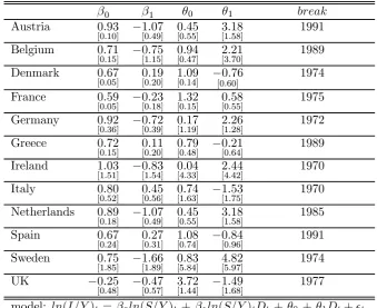
(cf. Table 1B) that with a panel of 12 units power must be expected to be rather low, such p-values should nevertheless be regarded as small enough to grant rejection. We can thus appreciate how applying the panel proce-dure does grant a power gain with respect to the individual tests, allowing to reach the more plausible conclusion that in this group of countries in-vestment and savings do seem to be linked by a long-run relationship, but this is likely to have changed over time at least once. The next natural step is to estimate models allowing for coefficient breaks at the estimated breakpoints btb
i = arg max(SupFbi). Given the small time sample available
this case there may not be an actual causal link of any relevance running from domestic savings to investment. Finally, in the four remaining cases (Italy, Spain, Greece, Denmark), contrary to expectations, the retention ratio seems to increase. However, two remarks are in order: first, the asso-ciated coefficient is never significant (nor the individual stability statistics, with the exception of Greece); second, in two cases (Italy and Spain) the estimated break points falls at the extremes of the interval in which they are constrained to lie (respectively, 1970 and 1991). From Fig. 2 we know that this is typical of cases when no break actually took place. Unfortunately, with the available sample size no reliable conclusions for individual cases can be reached, so it is impossible to shed more light on the issue. Clearly, the great care invoked above is fully necessary.
Fig. 3A. Savings (S) and Investments (I) to GDP (Y) ratios dynamics, 1960-2002. Top to bottom: Austria, Belgium, Denmark, Finland, France,
Germany, Greece. Left Column: S/Y (solid line) and I/Y (dotted line). Right Column: Current Account/GDP = (S−I)/Y (solid line) and zero
Fig. 3B. Savings (S) and Investments (I) to GDP (Y) ratios dynamics, 1960-2002. Top to bottom: Ireland, Italy, Netherlands, Portugal, Spain, Sweden, UK.Left Column: S/Y (solid line) and I/Y (dotted line). Right Column: Current Account/GDP = (S−I)/Y (solid line) and zero (dotted
Table 7
Investment and Savings to GDP ratios: ADF Unit Root Tests
Austria Belgium Denmark Finland France Germany Greece
I −1.31 −1.57 −1.42 −2.16 −1.26 −2.00 −2.13
S −0.62 −1.46 −2.03 −3.34∗ −1.49 −1.66 −1.11 Ireland Italy Netherlands Portugal Spain Sweden UK
I −2.34 −1.32 −1.11 −3.42 −2.93 −1.54 −2.16
[image:24.595.141.508.309.422.2]S −1.85 −1.29 −1.94 −4.87∗∗ −2.42 −2.06 −0.79 *: significant at 5%; **: 1%.
Table 8
Individual stability tests of the investment-savings long-run relationship, 1960-2002
Austria Belgium Denmark France Germany Greece Lc 0.27 1.28∗∗∗ 0.12 0.08 0.26 0.35
M eanF 2.19 45.15∗∗∗ 0.75 0.53 2.48 5.12∗∗ SupF 4.07 163.34∗∗∗ 1.65 1.18 10.94 27.52∗∗∗
Ireland Italy Netherlands Spain Sweden UK
Lc 0.25 0.19 0.22 0.17 0.17 0.05
M eanF 3.17 1.23 1.86 1.51 4.90 0.75 SupF 14.57∗∗ 6.80 3.19 5.63 12.50 12.36 trimming: 12.5%;
*: significant at 10%; **: 5%;***: 1%.
Table 9
Panel tests of stability of the investment-savings long-run relationship, 1960-2002
p-values ×100
mean median
Trimming Lc M eanF SupF Lc M eanF SupF
25% 3.1 0.0 0.0 14.4 12.1 44.7 12.5% 3.4 0.0 0.0 16.7 14.9 0.2
panel: Austria, Belgium, Denmark, France, Germany, Greece, Ireland, Italy, Netherlands, Spain, Sweden, UK;
[image:24.595.134.457.514.578.2]Table 10
The investment-savings long-run relationship, 1960-2002
FM-OLS estimates
β0 β1 θ0 θ1 break
Austria 0.93
[0.10] −1.07[0.49] 0.45[0.55] 3.18[1.58] 1991
Belgium 0.71
[0.15] −0.75[1.15] 0.94[0.47] 2.21[3.70] 1989
Denmark 0.67
[0.05] 0.19[0.20] [01.09.14] −[00.76.60] 1974
France 0.59
[0.05] −0.23[0.18] 1.32[0.15] 0.58[0.55] 1975
Germany 0.92
[0.36] −0.72[0.39] 0.17[1.19] 2.26[1.28] 1972
Greece 0.72
[0.15] 0.11[0.20] [00.79.48] −0.21[0.64] 1989
Ireland 1.03
[1.51] −0.83[1.54] 0.04[4.33] 2.44[4.42] 1970
Italy 0.80
[0.52] 0.45[0.56] [10.74.63] −1.53[1.75] 1970
Netherlands 0.89
[0.18] −1.07[0.49] 0.45[0.55] 3.18[1.58] 1985
Spain 0.67
[0.24] 0.27[0.31] [01.08.74] −0.84[0.96] 1991
Sweden 0.75
[1.85] −1.66[1.89] 0.83[5.84] 4.82[5.97] 1974
UK −0.25
[0.48] −0.47[0.57] [13.72.44] −1.49[1.68] 1977
model: ln(I/Y)t= β0ln(S/Y)t +β1ln(S/Y)tDt +θ0 +θ1Dt+²t,
Dt= 1 ift > break,0 else;
standard errors in brackets.
5
Conclusions
6
References
Bai J., Ng S. 2004 ”A PANIC Attack on Unit Roots and Cointegration” Econometrica 72, 1127-1177.
Banerjee, A., Carrion-i-Silvestre J.L. (2004) ”Breaking Panel Cointegra-tion”,Mimeo, European University Institute.
Banerjee, A., Carrion-i-Silvestre J.L. (2006) ”Cointegration in Panel Data With Breaks and Cross-Section Dependence”, Working Paper Series
n. 591, European Central Bank.
Bewley, R.A. (1979) ”The Direct Estimation of the Equilibrium Response in Linear Models”Economics Letters, 3, 375-381.
Engle, R.F and C.W.J. Granger (1987) ”Co-integration and Error Cor-rection: Representation, Estimation and Testing”, Econometrica, 55, 251-176.
Emerson, J., Kao, C. (2001) ”Testing for Structural Change of a Time Trend Regression in Panel Data: part I”, Journal of Propagations in Probability and Statistics, 2, 57-75.
Emerson, J., Kao, C. (2005) ”Bootstrapping and Hypothesis Testing in Non-Stationary Panel Data”Applied Economics Letters, 2005, 12, 313-318.
Fachin, S. (2006) ”Long-Run Trends in Internal Migrations in Italy: a Study in Panel Cointegration with Dependent Units”,Journal of Ap-plied Econometrics, forthcoming.
Gengenbach, C., Palm, F., Urbain, J.P. (2005) ”Panel Cointegration Test-ing in the Presence of Common Factors”, Paper presented at the Con-ference on Frontiers in Times Series Analysis, Olbia.
Gregory, A.W., Nason, J.M., Watt, D. (1996) ”Testing for Structural Breaks in Cointegrated Relationships”, Journal of Econometrics, 71, 321-341.
Gutierrez, L. (2005) ”Tests for Cointegration in Panels with Regime Shifts”,
Mimeo,Department of Agricultural Economics, University of Sassari.
Hansen, B.E. (1992) ”Tests for Parameter Instability in Regressions with I(1) Processes”,Journal of Business and Economic Statistics, 10, 321-335.
Kao, C., Chiang, M-H. (2000) ”Testing for Structural Change of a Cointe-grated Regression in Panel Data”Mimeo, Center for Policy Research,
Syracuse University.
Obstfeld, M. and Rogoff, K. (2000) ”The Six Major Puzzles in International Macroeconomics: Is There a Common Cause?” NBER Working Paper Series n. 7777.
Pedroni, P. (1999) ”Critical Values for Cointegration Tests in Heteroge-neous Panels with Multiple Regressors”,Oxford Bulletin of Economics and Statistics, 61, 653-670.
Pedroni, P. (2004) ”Panel Cointegration, Asymptotic and Finite Sample Properties of Pooled Time Series tests with an Application to the PPP hypothesis”,Econometric Theory, 20, 597-625.
Pesaran, M.H. (2006) ”A Simple Panel Unit Root Test in the Presence of Cross Section Dependence”,DAE Working Paper No. 0346, Cam-bridge University.
Politis, D.N., Romano, J.P. (1994) ”The Stationary Bootstrap”, Journal of the American Statistical Association, 89, 1303-1313.
Politis, D. N., White, H. (2003) ”Automatic Block-Length Selection for the Dependent Bootstrap”,Econometric Reviews, 23, 53-70.
Westerlund, J. (2006) ”Testing for Panel Cointegration with Multiple Struc-tural Breaks”, Oxford Bulletin of Economics and Statistics, 68, 101-132.