Estimation of a preference based single index from the sexual quality of life questionnaire (SQOL) using ordinal data

Munich Personal RePEc Archive

Estimation of a preference based single

index from the sexual quality of life

questionnaire (SQOL) using ordinal data

Ratcliffe, J and Brazier, J and Tsuchiya, A and Symonds, T

and Brown, M

The University of Sheffield

November 2006

HEDS Discussion Paper 06/06

Disclaimer:

This is a Discussion Paper produced and published by the Health Economics and Decision Science (HEDS) Section at the School of Health and Related Research (ScHARR), University of Sheffield. HEDS Discussion Papers are intended to provide information and encourage discussion on a topic in advance of formal publication. They represent only the views of the authors, and do not necessarily reflect the views or approval of the sponsors.

White Rose Repository URL for this paper:

http://eprints.whiterose.ac.uk/11031/

Once a version of Discussion Paper content is published in a peer-reviewed journal, this typically supersedes the Discussion Paper and readers are invited to cite the published version in preference to the original version.

Published paper

Ratcliffe J, Brazier J, Tsuchiya A, Symonds T, Brown M. Using DCE and ranking data to estimate cardinal values for health states for deriving a preference-based single index from the sexual quality of life questionnaire. Health Economics [in press].

The University of Sheffield

ScHARR

School of Health and Related Research

Health Economics and Decision Science

Discussion Paper Series

November 2006

Ref: 06/6

Estimation of a preference based single index

from the sexual quality of life questionnaire (SQOL) using ordinal

data.

Ratcliffe J1, Brazier J1, Tsuchiya A1, Symonds T2, Brown, M2

1. Health Economics and Decision Sciences, ScHARR,

University of Sheffield

2. Worldwide Outcomes Research, Pfizer Global

Pharmaceuticals, Pfizer Ltd

Corresponding Author: Julie Ratcliffe

Health Economics and Decision Science School of Health and Related Research University of Sheffield

Regent Court, Sheffield, UK S1 4DA

Email: [email protected]

Abstract

There is increasing interest in using ordinal methods to estimate cardinal

values for health states to calculate quality adjusted life years. This paper

reports the estimation of models of rank data and discrete choice experiment

(DCE) data to derive a preference-based index from a condition specific

measure relating to sexual health and to compare the results to values

generated from time trade-off valuation (TTO). The DCE data were analysed

using a random effects probit model and the DCE predicted values were

re-scaled according to the highest and lowest predicted TTO values

corresponding to the best and worst SQOL health states respectively. The

Rank data were analysed using a rank ordered logit model and re-scaled

using two alternative methods. Firstly, re-scaling the rank predicted values

using identical methods to those employed for DCE and secondly, re-scaling

the rank model coefficients by dividing each level coefficient by the coefficient

relating to death. The study raises some important issues about the use of

1. Introduction

Health state values are usually obtained using cardinal methods such as

standard gamble (SG), time trade-off (TTO) or visual analogue scaling (VAS).

However, there are a number of concerns with these techniques (Brazier et al,

1999). The direct and choice-less nature of the VAS task has been criticised

(Bleichrodt and Johannesson 1997) and VAS data may be subject to end

point and context bias (Torrance et al, 2001). Although SG and TTO are often

identified as preferred over VAS due to their choice based theoretical

underpinnings (Brazier et al, 2006), the values produced by these methods

are influenced by factors beyond the respondents preference for the health

state including time preference, risk attitude and loss aversion (Bleichrodt,

2002) . For these reasons, there is increasing interest in using ordinal

methods to estimate cardinal values for health states to calculate quality

adjusted life years

Until very recently, the use of ordinal data in health state valuation such as

from ranking or discrete choice experiments (DCE) has largely been ignored.

Ranking exercises have traditionally been included in health state valuation

studies as a warm up procedure to familiarise the respondent with the set of

health states to be valued and with the relative value of health states. Often

these data may not be used at all in data analysis, or they may be used to

check consistency between the ordinal ranking of health states and the

ranking of health states according to their actual values obtained using a

theoretical basis for deriving cardinal values from rank preference data (Kind,

1996). Thurstone’s method considers the proportion of times that one health

state (A) is considered worse than another health state (B). The preferences

over the health states are represented by a latent cardinal utility function and

the likelihood of health state A being ranked above health state B when health

state B is actually preferred to health state A is a function of how close to

each other the states lie on this latent utility function.

Salomon (2003) used conditional logistic regression to model rank data from

the UK MVH valuation of the EQ-5D. He was able to estimate a model that

was comparable to the original TTO model by rescaling the worst state using

the observed TTO value. Other methods of rescaling were also considered,

including normalization to produce a utility of 0 for death, but these were

found not to provide the best fitting predictions. McCabe et al (2006), using

similar methods, presented evidence to suggest that rank data that produced

cardinal health state valuation models for two generic measures of health

status, the HUI2 and SF-6D, were very similar to the original SG models.

DCEs have their theoretical basis in random utility theory (McFadden, 1973;

Hanemann, 1984; Ryan 1996). Although DCEs have become a very popular

tool for eliciting preferences in health care, the vast majority of published

studies using DCE methodology have tended to focus upon the possibility that

individuals derive benefit from non-health outcomes and process attributes in

addition to health outcomes. A limited number of studies have used DCEs to

estimate values for different health state profiles (Hakim and Pathak, 1999;

to date have linked these values to the full-health dead scale required for the

calculation of QALYs.

This study sought to examine the potential of ranking and DCE data to

estimate a preference-based index for a condition specific measure related to

sexual quality of life, and to compare the results to models estimated using

TTO data and observed TTO health state values.

2. Methods

2.1. Sexual quality of life questionnaire

The sexual quality of life questionnaire (SQOL) was originally developed as a

measure of sexual quality of life for use in a clinical trial setting (Symonds et al

2005). The SQOL has 3 dimensions and 18 items with 6 responses each from

completely agree to completely disagree. Each dimension is scored by

summing the responses to each item (where each response is coded from

one: completely agree to six: completely disagree). In its current form SQOL

has a very limited role in assessing cost effectiveness. To extend the scope of

the SQOL for use in economic evaluation, values were required to be elicited for

health states derived from the SQOL in order to make it preference based .

The current SQOL would generate many millions of health states that would

be too large for valuation. The first task of this study was to derive a health

state classification amenable to valuation. A preliminary study was

(Brazier and Ratcliffe, 2004). The resultant health state classification system,

the SQOL-3D comprised three dimensions: sexual performance, sexual

relationship and sexual anxiety; with four levels attached to each dimension

(Table 1). A health state is formed by selecting one level from each dimension

and in this way 64 health states can be defined (i.e. 4*4*4) by the SQOL-3D .

Table 1 here

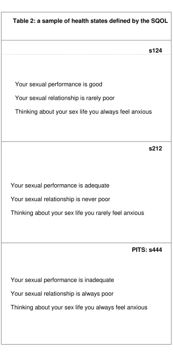
Each respondent was asked to value eight health states plus the PITS state -

the health state comprising the lowest level on each of the three dimensions

(see Table 2 for a sample of health states defined by the SQOL). These 64

states were grouped into 8 samples or blocks of 8 states to reflect a range of

health states defined by the classification rather than predominantly a ‘good’

or ‘bad’ selection of health states.

Table 2 here

2.2: Valuation survey

Interview

The aim was to interview a representative sample of 200 adult members of

the general population. Consenting adults were visited in their home by an

interviewer to conduct the valuation study. A small pilot study (n=18) was

undertaken in advance of the main study to check that interviewees

Prior to the elicitation of health state values using the TTO method,

respondents were asked to rank a set of health states from best to worst.

The ranking set contained 11 health states in total, the 9 health states

which were subsequently valued using the TTO (including the PITS state),

plus the best SQOL health state containing the most desirable levels on all

dimensions and immediate death. The second stage of the interview

involved obtaining TTO valuations of the health states defined by the

classification. The main valuation survey was undertaken using the

Measurement and Valuation of Health (MVH) group version of TTO with a

visual prop (MVH Group, 1995).

The TTO elicitation task asks people to imagine they will be in a state (j) for

10 years, and then asks them to consider a number of shorter periods in

perfect health (p). At the point where respondents are unable to choose

between state j and time period p in perfect health, the value of state j is given

as p/10. It is important to note that the upper anchor was therefore perfect

health and not the best state defined by the SQOL classification. This is

different from the valuation of generic preference based measures such as

the EQ-5D which used the best state defined by the EQ-5D classification. This

is because the best state defined by a condition specific measure like the

SQOL is not likely to be perfect health. For calculating QALYs it is necessary

to ensure that the results lie on the scale where 1 is perfect health and 0 is

equivalent to being dead. Respondents were initially taken through a practical

TTO to help them understand the task. They were then asked to undertake a

questions. Finally, they were asked whether they would be willing to

participate in a further postal survey.

Follow-up postal survey

In order not to over burden respondents at the interview, it was decided to

administer the DCE by post four weeks after the interview.

A computer programme developed by Huber and Zwerina (2000) used in the

statistical package SAS was applied to obtain an optimal statistical design for

the DCE based upon (i) level balance (ii) orthogonality (iii) minimum overlap

and (iv) utility balance. Such a design reduces the possible combinations of

attributes and their respective levels (or scenarios) to a manageable number

for the purposes of a mail out survey questionnaire whilst retaining maximum

statistical efficiency for the estimation of model parameters.

The programme produced 12 pairwise choices for comparison. The 12

pairwise choices were randomly distributed between two versions of the

questionnaire comprising 6 pairwise choices in each. For each health state

pair, respondents were asked to indicate which health state they considered

as better (see Appendix 1 for an example of a discrete choice question

included within one of the choice sets).

The two versions of the DCE questionnaire were randomly administered by

post to all consenting adults approximately four weeks after the completion

of the TTO interview. A reminder was sent out to all non-respondents

2.3. Data analysis - TTO

The data from the TTO valuation exercise were analysed using two main

approaches based upon aggregate and individual level modelling

respectively (Brazier et al, 2002). Firstly, ordinary least squares (OLS) was

used to estimate a mean level model: Model 1. The mean health state

values were the dependent variable and the independent variables were a

series of dummy explanatory variables representing each level of the three

dimensions of the SQOL. The mean level model is defined as:

Yi = f(β⁄xij) + Єi (1)

Where the dependant variable Yi is the value (mean TTO value) for each

health state (i) and xis a vector of dummy explanatory variables (x∂λ) for each

level λ of dimension ∂ of the simplified SQOL classification. For example, x31

denotes dimension ∂= 3 (sexual anxiety), level λ = 1 (thinking about your sex life you never feel anxious). For any given health state x∂λ will be defined as:

x∂λ=1, if for this state dimension ∂is at level λ

x∂λ =0, if for this state, dimension ∂is not at level λ

There are 9 of these terms in total with level λ = 1 acting as a baseline for each dimension. Hence for a simple linear model, the intercept (or constant)

represents state 111, and summing the coefficients of the ‘on’ dummies

derives the value for all other states. Єiis the error term which is assumed to

Secondly, a one way error components random effects model: Model 2 was

specified which takes account of the repeated measurement aspect of the

data whereby multiple responses are obtained from the same individual

(Diggle et al, 2002).

The random effects model is defined as (Brazier et al, 2002):

Yij = f(β’xij) + Єij (2)

Where i=1,2 …n represent individual health state values and j = 1,2…m

represents respondents. The dependant variable Yij is the disvalue (1-mean

TTO value) for health state i valued by respondent j, x is a vector of dummy

explanatory variables (x∂λ) defined as previously and Єij is the error term which

is subdivided as follows:

Єij = uj + eij (3)

Where uj is respondent specific variation and eij is an error term for the ith

health state valuation of the jth individual, and this is assumed to be random

across observations. A one way error components fixed effects model can

also be specified. This differs from the random effects specification in that the

respondent specific effects are not assumed to be random but are a set of

fixed effects to be estimated, together with the vector of coefficients on the

explanatory variables. The selection of the most appropriate model

specification was informed by the Hausman test (Hausman, 1978).

2.4 Data analysis: DCE

The data from the DCE survey were analysed using a random effects probit

equation (2). The estimated coefficients and their statistical significance (or

otherwise) indicate the relevant importance of the different levels of the

dimensions on individual preferences.

2.5 Data analysis: Ranking

The rank ordered logit model was used to analyse the ranking data: Model 4.

This model is based upon the assumption that the respondent makes a series

of selections from smaller and smaller groups. Thus in ranking 11 health

states (as was the case for this study with 9 states being valued plus full

health and immediate death) we assume that the respondent chooses the

most preferred state from the full set, then chooses the most preferred state

from the remaining 10 etc until all health states have been assigned a rank

between 1 and 11. The independence of irrelevant alternatives assumption is

required to characterise this process as equivalent to a series of pairwise

choices i.e. the ranking of the pair is not affected by the other states that are

ranked in the same exercise (Luce, 1959).

The rank ordered logit model states that respondent j has a latent utility

function for state i, Uji and given the choice of two states i and k, the

respondent will choose state i over state k if Uji > Ujk.

The expected value of each unobserved utility was assumed to be a linear

function of the categorical levels on the dimensions of the SQOL. Following

the approach taken by Salomon (2003) and McCabe et al (2006), the general

= µ + єij where µj is representative of the tastes of the population and єij

represents the particular tastes of the individual. If the error term є has an extreme value distribution, then the odds of choosing state j over state k are

exp{µj - µk}.

2.6 Scaling

The DCE and rank model values (Models 3 and 4) produce predicted

valuations on an interval scale such that meaningful comparisons of

differences are possible but the origins and units of the scale are defined

arbitrarily by the identifying assumptions in the model (Salomon, 2003). In

order to infer cardinal valuations from the DCE and rank models on a scale

where zero is dead and one is perfect health it is necessary to re-scale the

estimated valuations for health states. Two alternatives were considered.

Firstly, re-scaling both the rank and DCE predicted values such that the

lowest value (relating to the PITS state) was anchored at the lowest value for

the PITS state predicted by the mean level TTO model (0.672) and the

highest value (relating to the best SQOL heath state) was anchored at the

highest value for the best SQOL state predicted by the mean level TTO model

(0.946). Secondly, re-scaling the rank model coefficients by dividing each

level coefficient by the coefficient relating to death: Model 5. This re-scaling

option normalises the rank data to produce a utility value of 0 for death

(Salomon, 2003). Unfortunately, this method could not be used to re-scale the

DCE data also since none of the pairwise health state comparisons included

2.4 Results

Out of the 376 useable addresses contacted for interview, 207 individuals

agreed to participate (a 55% response rate). For the DCE postal follow up

survey a response rate of 49% was achieved (102/207) after one reminder.

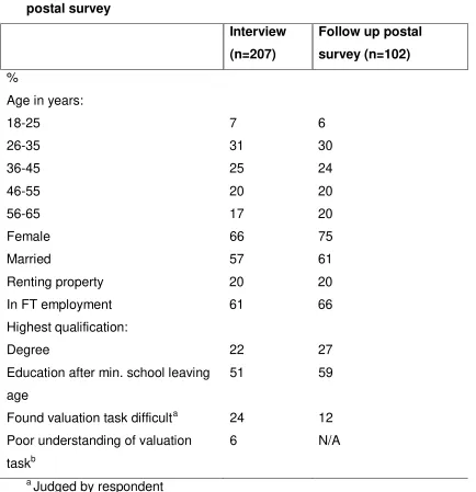
The characteristics of the respondents to the interview and the follow up

postal survey respectively are presented in Table 3. The characteristics of

respondents to both the interview and the survey were broadly similar with the

majority of respondents being female, married and in full-time employment.

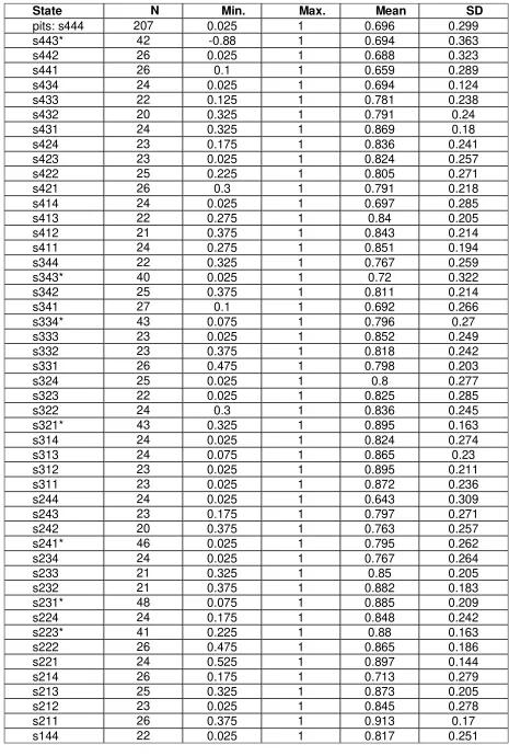
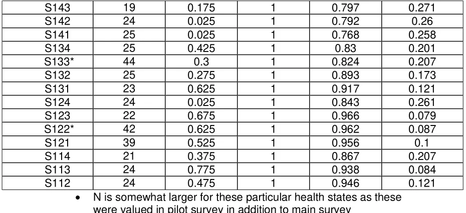
Descriptive statistics for the 64 health states are presented in Table 4. Mean

TTO health state values range from 0.643 to 0.966 and standard deviations

between 0.10 and 0.36. Most health states had 20-30 observations with the

PITS state having 207 (i.e. all respondents).

Table 3 here

Table 4 shows the results for the mean and random effects models for the

TTO, the DCE and ranking models. The dimension level dummies represent

progressively worse problems on each dimension compared to the baseline.

As such the coefficient estimates are expected to be negative and increasing

in absolute size. An inconsistent result occurs where a coefficient on the main

effects dummies decreases in absolute size with a worse level.

For the mean level TTO (Model 1) all of the coefficients have the expected

negative sign, with the exception of the movement from level 1 to level 2 in

sexual relationship which is positive (though very small and not signficant).

Five of the 9 dimension level coefficients are statistically significant (p<0.05),

along with the constant term. With the exception of level 2 to 3 of the

dimension relating to sexual performance, the coefficient estimates increase

with absolute size as the level of each dimension worsens. The explanatory

power of the mean level model is 0.517.

The Hausman test suggests that random, rather than fixed effects is the most

appropriate model specification (Chi2 = 7.50 p Chi2 = 0.221). For the random

effects TTO (Model 2) the results are quite similar in that all of the coefficients

have the expected negative sign and increase with size as the level worsens.

In total, 8 of the 10 coefficients are statistically significant (p<0.05).

The ability of the mean level TTO model to predict observed TTO values is

superior to the random effects model, resulting in fewer errors greater than

0.05 and 0.10 in absolute value. Furthermore, the mean model has a mean

absolute error (MAE) of 0.040 compared to 0.072. In both models the

predictions are unbiased (t-test) indicating that neither model systematically

over or under estimates the observed mean TTO. However, the Ljung-Box

(LB) statistics reveal auto correlation in the prediction errors of both models,

when the errors are ordered by actual mean health state valuation.

For the DCE model (Model 3), all of the coefficients have the expected

The coefficient estimates increase with absolute size as the level of each

dimension worsens with the exception of the movement from level 2 to level 3

in sexual anxiety (although this inconsistency is small and does not relate to

statistically significant dimension levels). For the rank ordered logit models:

Models 4 and 5 the results have the expected negative sign and increase with

size as the level worsens with the exception of the movement from level 1 to

level 2 in sexual anxiety. In total, 9 of the 10 coefficients are statistically

significant (p<0.05).

The ability of the DCE and ranking models to predict observed mean TTO is

broadly similar both in terms of their MAEs compared to observed mean TTO

and in the number of differences compared to observed TTO greater than

0.05 and 0.10 in absolute value. In contrast to the TTO models, the DCE and

both ranking models produce biased predictions (t-test). The LB test found

evidence of a systematic pattern in the differences of the predictions from the

ranking model though not the DCE model. As would be expected, neither the

ranking or DCE models perform as well as the mean level TTO model in

terms of their ability to replicate TTO observed values.

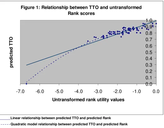
Figure 1 illustrates how re-scaling the raw rank predicted values (Model 4)

according to the predicted TTO values for the best and worst SQOL health

state effectively assumes a linear relationship and fits the predicted mean

level TTO values well. However, probably because even the worst SQOL

health is relatively mild in terms of severity, this method of re-scaling does not

to produce a value of 0 for death (Model 5) the predicted values for the rank

data do not correspond as well to the mean level TTO values.

Figure 1 here

The predictions of Models 1-5 are compared graphically in Figures 2-6. The

health states have been ordered simply in terms of their state number, with

444 at the start as the most severe state (i.e. level 4 on all dimensions) to the

best state 111. This does not represent a monotonic scale, but broadly

speaking the value of states increases when moving from left to right along

the horizontal axis. It can be seen from Figure 2 that values predicted by the

mean level TTO model (model 1) follow fairly closely the observed TTO

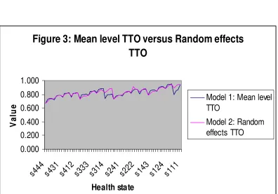
values, with no discernible pattern. Figure 3, suggests very little differences

between the RE TTO (model 2) and the mean level TTO values where as the

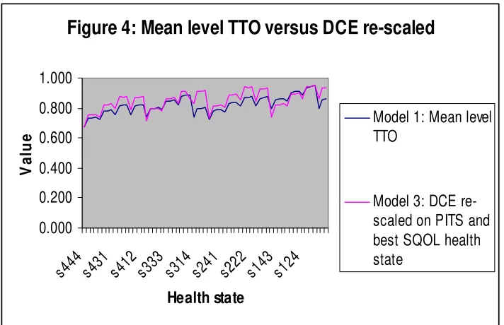
mean level TTO values lie above the DCE values re-scaled according to the

values for the pits and best SQOL health states (Model 3) for the vast majority

of states (Figure 4). By contrast, the rank values re-scaled in an identical

manner (Model 4) shown in Figure 5 lie below the predicted TTO values for

more severe states and converge towards the predicted mean TTO values at

very mild states with the exception of the PITS state and the best SQOL

health states which are set to be equal. When the rank values are re-scaled

using death as the bottom anchor (Model 5), the results, presented in Figure

6, indicate that the re-scaled rank values lie markedly below the predicted

TTO values for more severe states and above the predicted TTO values for

Figures 2-6 here

Finally, we have examined the ability of the models to predict the logical

ordering of pairs of SQOL states, where one state should be preferred to

another because it is better on at least one dimension, but no worse on any

other dimension. In this respect we found that both the mean level TTO

(model 1) and the random effects TTO (model 2) performed best with no

logical inconsistencies whereas the ordinal models fare worst with the DCE

(model 3) exhibiting 7 logical inconsistencies and rank models (models 4 and

5) having 17 and 15 logical inconsistencies respectively.

3. Discussion

The paper has presented the results of estimating a preference-based index

for a condition specific health state classification using rank and DCE data

and comparing the results to a conventional TTO model. Previous research

has used rank data, but to our knowledge this is the first study to use DCE

data to estimate health states values on the full health-dead scale required to

calculate QALYs.

As would be expected the TTO models faired better than the ordinal models in

replicating observed TTO valued. The RE TTO model (2) performed only

slightly better than the rank (4 and 5) and DCE models (3) in terms of MAE.

However, the latter two models suffered from the presence of bias and

from modelling rank data for the HUI2 and SF-6D where the rank data were

broadly comparable to actual SG (McCabe et al, 2006), though the analysis of

rank data for the EQ-5D found differences for the rescaling against being

dead (check Salomon, 2004). As commented on in McCabe et al (2006),

there is no reason why models estimated from ordinal data should generate

the same values as those produced by conventional cardinal methods. More

research is needed to compare ordinal and cardinal methods, but these

results support the view that they do generate different values.

This paper has also compared the ability of TTO to predict the logical

orderings of health states compared to the ordinal methods. It might be

expected that models estimated from ordinal data would perform better in this

regard. However, the random effects TTO model performed best. This may be

due to the biases found in both the DCE and ranking models

This study has highlighted a number of methodological issues which warrant

further investigation. In relation to the ranking data analysis, the

independence of irrelevant alternatives assumption which characterises the

selection process as equivalent to a series of pairwise choices and assumes

that the ranking of the pair is not affected by the other states that are ranked

in the same exercise is a strong assumption which may be criticised as

unrealistic (McCabe et al, 2006). In this respect, other variants of ordinal and

discrete choice data collection strategies which do not rely upon this

assumption, e.g. best worst scaling (Marley and Louviere, 2005) warrant

further investigation in a health care context. In addition, further empirical

by ordinal valuation techniques to framing effects that may produce significant

differences in responses including subtle variants in question wording, context

and modes of administration.

We found that the two ordinal methods produced different results. DCE data

produced substantially higher values than the ranking data. However, it can

be argued that the DCE values were not based upon a ‘pure’ test of this

method since the values were anchored externally using the predicted TTO

value for the PITS and best SQOL health states. The DCE was administered

by post following the TTO interviews and so the respondents were ‘warmed

up’ in that they were already familiar with the health states to be compared.

Furthermore, only a sub- sample responded to the postal survey although

they were broadly similar in characteristics to respondents from the main

interview study.

Ordinal measurement strategies such as ranking or DCE may have

considerable practical advantages over TTO and SG because it can be

argued that they place a lower cognitive burden on respondents and do not

require such a high degree of abstract reasoning. However, this assertion

needs to be subject to further research. In addition ordinal measurement

strategies are not contaminated by issues relating to time preference or

attitudes to risk, factors affecting TTO and SG generated health states values

respectively. Further empirical studies are required to more fully determine the

Whilst re-scaling the raw rank and DCE predicted values in reference to the

lowest and highest predicted TTO values (Models 3 and 4) provided better

fitting estimates in this study than re-scaling the rank model coefficients in

reference to the value for death (Model 5), fixing the scale in reference to a

value of zero for death may be considered more appropriate in facilitating

normalisation on a scale that will enable the estimation of QALY’s because it

does not need to rely upon information derived from another valuation method

(i.e. TTO). In this respect, the inclusion of the state dead within the DCE

pairwise health state comparisons would also enable this method of re-scaling

to be employed for DCE data. However, it should also be noted that for

condition specific instruments where the worst health state appears relatively

mild on the full health death scale, this approach can be problematic, as was

found with the SQOL. Further empirical work is required to investigate the

optimal method of re-scaling raw rank and DCE predicted values for generic

and condition specific instruments and the extent to which this may vary

References

Brazier JE, Deverill M, Harper R, Booth A (1999). A review of the use of

health status measures in economic evaluation. Health Technology and

Assessment 3 (9).

Brazier J, Ratcliffe J (2004). Survey comparing original response choices to

items of the SqoL to the levels of the SQoL state classification – Preliminary

findings. Report for Pfizer limited.

Brazier J, Ratcliffe J, Salomon J, Tsuchiya A (2006). The measurement and

valuation of health benefits for economic evaluation. Oxford University Press,

Oxford.

Brazier J, Roberts J, Deverill M. The estimation of a preference based single

index measure for health from the SF-36 (2002). Journal of Health Economics

21: 271-292.

Brazier J, Tsuchiya A, Busschbach J, Stolk E (2002). Issues in estimating a

preference based index for condition specific measures. Presentation at the

International Health Economics Association meeting, San Francisco, USA.

Brooks R, Rabin R, De Charro F (2004). The measurement and valuation of

health status using EQ-5D: a European perspective. Kluwer Academic

publishers, London.

Diggle PJ, Heagerty P, Liang KY, Zeger SL (2002). Analysis of longitudinal

data (2nd edition). Oxford University Press, Oxford.

Dowie J (2002). Decision validity should determine whether a generic or

condition specific HRQOL measure is used in health care decisions. Health

Feeny DH, Furling WJ, Torrance GW et al (2002). Multiattribute and single

attribute utility function – the health utility index mark 3 system. Medical Care

40: 113-128.

McCabe C, Brazier J, Gilks P, Tsuchiya A, Roberts J, O’Hagan A, Stevens K

(2006). Using rank data to estimate health state utility models. Journal of

Health Economics 25(3): 418-431.

MVH Group (1995). The measurement and valuation of health: Final report on

the modelling of valuation tariffs. Centre for Health Economics, University of

York.

Propper C (1995).The disutility of time spent on the United Kingdom’s

National Health Service waiting lists. The Journal of Human Resources, 30:

677-700.

Revicki DA, Leidy NK, Brennan-Diemer F et al (1998). Integrating patients

preferences into health outcomes assessment: the multiattribute asthma

symptom utility index. Chest 114: 998-1007.

Ryan M, Farrar S (1994). A pilot study of using conjoint analysis to establish

the views of users in provision of orthodontic services in Grampian. Health

Economics Research Unit Discussion Paper 07/94. University of Aberdeen,

Aberdeen.

Ryan M (1996). The application of conjoint analysis in health care. Office of

Health Economics publications, London.

Salomon JA (2003) Reconsidering the use of rankings in the valuation of

health states: a model for estimating cardinal values from ordinal data.

Salomon JA, Murray CJ (2004). A multi-method approach to measuring health

Stolk EA, Busschbach JJV (2003). Validity and feasibility of the use of

condition specific outcome measures in economic evaluation. Quality of Life

Appendix 1: Example of choice question included in DCE questionnaire

Pair 1

Health State A Health State B

Your sexual performance is good Your sexual performance is adequate

Your sexual relationship is never poor Your sexual relationship is rarely poor

Thinking about your sex life you some times feel anxious

Thinking about you sex life you rarely feel anxious

Which health state do you think is better? (please tick one box only)

Table 1: Dimensions and levels chosen for the simplified SQOL

classification

1. Sexual performance

• Your sexual performance is good

• Your sexual performance is adequate

• Your sexual performance is sometimes inadequate

• Your sexual performance is inadequate

2. Sexual relationship

• Your sexual relationship is never poor

• Your sexual relationship is rarely poor

• Your sexual relationship is sometimes poor

• Your sexual relationship is always poor

3. Sexual anxiety

• Thinking about your sex life you never feel anxious

• Thinking about your sex life you rarely feel anxious

• Thinking about your sex life you sometimes feel anxious

Table 2: a sample of health states defined by the SQOL

s124

Your sexual performance is good

Your sexual relationship is rarely poor

Thinking about your sex life you always feel anxious

s212

Your sexual performance is adequate

Your sexual relationship is never poor

Thinking about your sex life you rarely feel anxious

PITS: s444

Your sexual performance is inadequate

Your sexual relationship is always poor

Table 3 : Characteristics of respondents to interview and follow up

postal survey

Interview

(n=207)

Follow up postal

survey (n=102)

%

Age in years:

18-25 7 6

26-35 31 30

36-45 25 24

46-55 20 20

56-65 17 20

Female 66 75

Married 57 61

Renting property 20 20 In FT employment 61 66 Highest qualification:

Degree 22 27

Education after min. school leaving age

51 59

Found valuation task difficulta 24 12 Poor understanding of valuation

taskb

6 N/A

a

Judged by respondent

b

Table 3: Descriptive statistics for the TTO valuations of the SQOL-3D

State N Min. Max. Mean SD

pits: s444 207 0.025 1 0.696 0.299

s443* 42 -0.88 1 0.694 0.363

s442 26 0.025 1 0.688 0.323

s441 26 0.1 1 0.659 0.289

s434 24 0.025 1 0.694 0.124

s433 22 0.125 1 0.781 0.238

s432 20 0.325 1 0.791 0.24

s431 24 0.325 1 0.869 0.18

s424 23 0.175 1 0.836 0.241

s423 23 0.025 1 0.824 0.257

s422 25 0.225 1 0.805 0.271

s421 26 0.3 1 0.791 0.218

s414 24 0.025 1 0.697 0.285

s413 22 0.275 1 0.84 0.205

s412 21 0.375 1 0.843 0.214

s411 24 0.275 1 0.851 0.194

s344 22 0.325 1 0.767 0.259

s343* 40 0.025 1 0.72 0.322

s342 25 0.375 1 0.811 0.214

s341 27 0.1 1 0.692 0.266

s334* 43 0.075 1 0.796 0.27

s333 23 0.025 1 0.852 0.249

s332 23 0.375 1 0.818 0.242

s331 26 0.475 1 0.798 0.203

s324 25 0.025 1 0.8 0.277

s323 22 0.025 1 0.825 0.285

s322 24 0.3 1 0.836 0.245

s321* 43 0.325 1 0.895 0.163

s314 24 0.025 1 0.824 0.274

s313 24 0.075 1 0.865 0.23

s312 23 0.025 1 0.895 0.211

s311 23 0.025 1 0.872 0.236

s244 24 0.025 1 0.643 0.309

s243 23 0.175 1 0.797 0.271

s242 20 0.375 1 0.763 0.257

s241* 46 0.025 1 0.795 0.262

s234 24 0.025 1 0.767 0.264

s233 21 0.325 1 0.85 0.205

s232 21 0.375 1 0.882 0.183

s231* 48 0.075 1 0.885 0.209

s224 24 0.175 1 0.848 0.242

s223* 41 0.225 1 0.88 0.163

s222 26 0.475 1 0.865 0.186

s221 24 0.525 1 0.897 0.144

s214 26 0.175 1 0.713 0.279

s213 25 0.325 1 0.873 0.205

s212 23 0.025 1 0.845 0.278

s211 26 0.375 1 0.913 0.17

Table 3: Descriptive statistics for the TTO valuations of the SQOL-3D (cont.)

S143 19 0.175 1 0.797 0.271

S142 24 0.025 1 0.792 0.26

S141 25 0.025 1 0.768 0.258

S134 25 0.425 1 0.83 0.201

S133* 44 0.3 1 0.824 0.207

S132 25 0.275 1 0.893 0.173

S131 23 0.625 1 0.917 0.121

S124 24 0.025 1 0.843 0.261

S123 22 0.675 1 0.966 0.079

S122* 42 0.625 1 0.962 0.087

S121 39 0.525 1 0.956 0.1

S114 21 0.375 1 0.867 0.207

S113 24 0.775 1 0.938 0.084

S112 24 0.475 1 0.946 0.121

• N is somewhat larger for these particular health states as these

30 Table 4: Comparison of mean level TTO, random effects TTO, DCE and Ranking model results

Model 1: Mean level TTO

Model 2: Random effects TTO Model 3: Random effects DCE Model 4: Rank ordered logit

Model 5: Rank ordered logit

re-scaled utility value of death = 0

Lev2 performance -0.072* -0.064* -0.095*

-0.735* -0.110*

Lev3 performance -0.060* -0.069* -0.308

-0.998* -0.149*

Lev4 performance -0.126* -0.127* -0.712*

-1.726* -0.258*

Lev2 relationship 0.001 -0.010 -0.052

-0.187 -0.028

Lev3 relationship -0.035 -0.042* -0.458*

-0.181* -0.027*

Lev4 relationship -0.084* -0.111* -1.183*

-0.975* -0.146*

Lev2 anxiety -0.002 -0.001 -0.076

-0.482 -0.072

Lev3 anxiety -0.009 -0.028* -0.071

-0.406* -0.061*

Lev4 anxiety -0.065* -0.060* -0.904*

-0.812* -0.121*

Constant 0.946* 0.961* 0.070

N/A N/A

Death dummy

N/A N/A N/A -6.685* -1.000*

N 64 207 64 189 189

Inconsistencies1 1 0 0 0 0

MAE (compared to actual TTO)_

0.037 0.072 0.077 0.069 0.083

Adjusted R2 0.517 0.207 0.203 0.198 0.198

No. > 0.05 19 (30%) 19 (30%) 18 (28%) 20 22 (34%)

No. > 0.10 45 (70%) 38 (60%) 45 (70) 42 (66%) 44 (69%)

t (mean=0) -0.301

(p=0.765) 0.942 (p=0.439) -13.664 (p=<0.001) -9.465 (p=<0.001) -7.227 (p=<0.001)

LB 4.099

(p=0.848) 86.21 (p=<0.001) 10.568 (p=0.227) 36.120 (p=0.076) 63.973 (p=<0.001)

Figure 1: Relationship between TTO and untransformed

Rank scores

0.0

0.1

0.2

0.3

0.4

0.5

0.6

0.7

0.8

0.9

1.0

-7.0

-6.0

-5.0

-4.0

-3.0

-2.0

-1.0

0.0

Untransformed rank utility values

p

re

d

ic

ted

T

T

O

_______Linear relationship between predicted TTO and predicted Rank

32

Figure 2: Mean level TTO versus

observed TTO

0.000 0.200 0.400 0.600 0.800 1.000

s

444 _s431 _s412 _s333 _s314 _s241 _s222 _s143 _s124 _s111

Health state

V

a

lu

e Model 1: Mean_{level TTO}

Observed TTO Values

Figure 3: Mean level TTO versus Random effects

TTO

0.000 0.200 0.400 0.600 0.800 1.000

s444 s431 s412s333 s314 s241 s222 s143 s124 s111

Health state

V

a

lu

e Model 1: Mean level_TTO

33

Figure 4: Mean level TTO versus DCE re-scaled

0.000 0.200 0.400 0.600 0.800 1.000

s444 s431 s412 s333 s314 s241 s222 s143 s124

Health state

V

a

lu

e

Model 1: Mean level TTO

Model 3: DCE re-scaled on PITS and best SQOL health state

Figure 5: Mean level TTO versus Rank re-scaled

on PITS and best SQOL health state

0.000 0.200 0.400 0.600 0.800 1.000 s 4 4 4 s 4 3 1 s 4 1 2 s 3 3 3 s 3 1 4 s 2 4 1 s 2 2 2 s 1 4 3 s 1 2 4 s 1 1 1 Health state V a lu e

Model 1: Mean level TTO

34

Figure 6: Mean level TTO versus Rank re-scaled

on utility value of death = 0

0.000 0.200 0.400 0.600 0.800 1.000 s 4 4 4 s 4 3 1 s 4 1 2 s 3 3 3 s 3 1 4 s 2 4 1 s 2 2 2 s 1 4 3 s 1 2 4 s 1 1 1 Health state V a lu e

Model 1: Mean level TTO