Novel Approach to Estimate Motion Blur Kernel
Parameters and Comparative Study of Restoration
Techniques
Kishore R. Bhagat
Dept. Digital communication NRI Institute of Information Sci.&Technology,Bhopal, India
Puran Gour
Dept. Digital communication NRI Institute of Information Sci.&Technology,Bhopal, India
ABSTRACT
Motion blur occurs due to the fact,that during exposure time there is movement of object or camera or both. Removing of blur is always challenging for image processing field because one has to estimate the motion blur which can spatially differ over image. Motion blur is simply an undesired effect. Restoration of blur image is very important in many of the cases like identification of criminal face in blurred image.In restoration of motion blur the knowledge of the point spread function (PSF) plays a vital role. This paper present a novel approach towards estimation of parameters like motion blur angle and the motion blur length which defines the PSF. Both of these parameters are used to restore the blurred image. Furthermore paper discusses the comparative study of different restoration techniques. The experimental result shows estimated blur angle and blur length are very close to theoretical value and the blur images with natural and artificial noise are successfully restored.
General Terms
Blur kernel parameters, Image fusion techniques,
Keywords
Image restoration, Image fusion PSF,Spectrum, Wiener.
1.
INTRODUCTION
Motion blur eventually causes degradation of image quality. The motion blur can be removed by minimizing the shutter exposure time but in case of low light situation this will causes unavoidable tradeoff of increased noise. One of the frequent reason of motion blur is camera shake. We can address this problem by using some mechanical means like camera can place on tripod stand. Secondly the object movement in the scene causes the motion blur. This type of blur is harder to control so it is often desirable to remove it by post synthesis of blur.
Images may be blur due to improper focusing of lens, atmospheric turbulence, undesirable working of optical systems, relative motion between the camera and scene. Hence in the restoration of noisy and blurred images knowledge of blurring system is important. Motion blur is defined with two essential parameters called motion blur angle and motion blur length. An Interactive Deblurring Technique for Motion Blur in which Segment based semi-automated restoration method is proposed using an error gradient descent iterative algorithm[1].R. Lokhande, K.V.
Aarya and P.Gupta [2] successfully proposed the algorithm to determine the motion blur PSF parameters.Numerous methods for estimation of blur parameters have been proposed in literature[3,4,5,6,7]. Fabian and Malah[4] discussed about the improvement in sensitivity of Cannon's method. Huiji& Chaoqiang Liu[5] introduce a hybrid Fourier-Radon transform to estimate the parameters of the blurring kernel with improved robustness to noise over available techniques. Gennery has discussed the parameters of blur function (PSF) in spectral domain[7]. Taeg Sang Cho has discussed about Blur Kernel Estimation using the Radon Transform[8]. Alex Rav-Acha, Shmuel Peleg[10] describes how different images, each degraded by a motion blur in a different direction, can be used to generate a restored image. Y. S. Chen and I. S. Choa describes transformation of the enhanced spectral magnitude function in cepstral domain[11] and the blurred image is pre-processed to remove the noise using Spectral Subtraction method[12] , whereas Cannon[17] has identified the point spread function (PSF) parameters in the power cepstrum of the image by inspecting the negative peak.
In most of the blur kernel parameter identification methods the blur motion is consider along the horizontal direction, in practice which is not always the case.The method of detecting the blur angle by rotating the coordinate system following by computing its 1-D spectrum and inspecting the peaks and valleys in it is discussed by Li and Yoshida[9].
This paper suggest the approach to find out motion blur PSF parameters, i.e. blur angle and blur length, in frequency domain. After getting the approximated parameters those are used in restoration of image. The different types of filters are used for restoration of images and have been compared in this paper. Further the wavelet based fusion is used for betterment of results.
Further this paper is organized as section 2 contains the Image Acquisition Model. Algorithms for identification of motion blur parameters have been explained in Section 3. The comparison of restoration method is given in Section 4. Section 5 contains the wavelet based image fusion. The experimental results are given in section 6. Finally conclusion is given.
Figure 1: Stages of proposed system
2.
IMAGE ACQUISITION MODEL
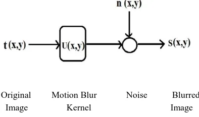
The technique for Image acquisition with linear space-invariant image system is depicted as shown in figure2. Mathematically represented as,
s(x, y) = t(x, y) * u(x, y) + n(x, y) (1)
Where t(x, y) is original image s(x, y) is the observed image; u(x, y) is the point spread function of the imaging system n(x, y) is additive noise which is Gaussian white noise with zero mean in our case and (*) is the convolution operator.If the u(x, y) point spread function is linear and space invariant function, then the blurred or noisy image is in spatial domain and it is given as,
𝑈 𝑥, 𝑦 =
1
𝑑, 𝑖𝑓 0 ≤ 𝑥 ≤ 𝑑; 𝑦 = 𝑑 cos ∅
0, 𝑂𝑡𝑒𝑟𝑤𝑖𝑠𝑒 (2)
Where d is blur length and it is proportional to relative velocity between camera and object to the exposure time.
Original Motion Blur Noise Blurred Image Kernel Image
Figure2: Image Acquisition System So s(x, y) also given as,
s(x, y) = t(x, y) * u(x, y) + n(x, y)
= 𝑀−1𝑖=0 𝑁−1𝑗 =0 𝑢 𝑥 − 𝑖, 𝑦 − 𝑗 𝑡 𝑥, 𝑦 + 𝑛(𝑥, 𝑦) (3) Where indicates the 2-D convolution and s, u, t and n are observed image, degradation function, original image and noise respectively. All of these images are of size MN, where M and N represent the image size in x and y axis respectively.
Above equation in the Fourier transform can be written as follows,
S (u, v) = T (u, v) .U (u, v) + N (u, v)(4)
Since convolution in spatial domain is multiplication in frequency domain.Where (u, v) are the spatial frequency coordinates and S,U,T and N represent the Fourier transforms of the observed image s, degradation function u, original image t and noise n respectively.
This paper deals with images blurred by the uniform linear motion between the image and the sensor during image acquisition. Consider the scene to be acquired at constant relative velocity V between the scene and the camera with an angle of degrees along the horizontal axis during the exposure time [0, T] then the motion blur PSF u(x, y) for blur length L = V T [10, 12] is given as in equation (2). For simplicity, let us assume that motion is along the horizontal direction i.e. = 0o
, then (2) can be expressed.
𝑢 𝑥, 𝑦 =
1
𝑑, 𝑖𝑓 0 ≤ 𝑥 ≤ 𝑑; 𝑦 = 0
0, 𝑂𝑡𝑒𝑟𝑤𝑖𝑠𝑒(5)
Using sin 𝑥 =2𝑗1 𝑒𝑗𝑥− 𝑒−𝑗𝑥 on the Fourier transform of (5) we will get,
𝑈 𝑘 = sin 𝑐 𝜋𝑘𝐿 . 𝑒−𝑗𝜋𝑘𝐿 (6)
The magnitude transfer function of (5) is given by
𝑈(𝑘) = sin 𝑐(𝜋𝑘𝐿)(7)
Note that U(k) is independent of the l (vertical frequency Coordinate). Similarly, the expression for motion blur PSF of blur length L whose blur angle is o
with the horizontal axis is obtained in [14] and given by,
𝑈 𝑘, 𝑙 = sin 𝑐 𝜋𝐿𝑡 ; 𝑤𝑒𝑟𝑒𝑡 = 𝑘 cos ∅ + 𝑙 sin ∅(8)
Above equation can be taken as model of PSF for given parameter l and.
3.
ESTIMATION OF BLUR KERNEL
FRAMEWORKS
In this section we discuss the line of action to find out the motion blur kernel parameters[2].
3.1
Blur Length Estimation
If noise is neglected, the Fourier transform of observed image is equal to the multiplication of Fourier transform of PSF (u(x, y)) and original image. The frequency response of the motion blur PSF(2) whose magnitude is given by (6), is characterized by periodic zeros on the k axis which occur at,
𝑘 = ±𝑑1, ±12𝑑, ±𝑑3, ±𝑑4… … .. (9)
Line of Action for Estimation of Blur Length
s x, y 𝐹𝑇 S k, l
Step2:The log spectrum of S(K, l) is calculated and converted to binary.
Step3: System coordinate of binary structure is rotated in direction opposite to the blur.
Step4:Convert the 2D data in single dimension by taking average along the columns
Step5:Take the IFT of 1-D data obtained in step 4. Step6:The real part of first negative value is found as
blur length.
Above algorithm is proposed with consideration of no noise. If noise is present the same steps to be followed by applying average filtering of blurred image before computing its Fourier transform. With assumption that that zero mean white Gaussian noise and average filter effectively remove the Gaussian noise [14].
3.2
Blur Angle Estimation
The spectrum of non-blurred original image is isotropic, whereas that of motion blurred image is anisotropic based on this observation on e can estimate the motion blur angle. u(x, y) is the convolution kernel that causes the motion blur so a blurred image due to motion is represented by a linear system of a convolution 𝑠 𝑥; 𝑦 = 𝑡 𝑥, 𝑦 𝑢(𝑥, 𝑦). The motion blur kernel low-passes the image in the direction of the blur. The anisotropy in the spectrum introduced by the motion blur is always perpendicular to the motion direction. Therefore, to determine the blur direction, the spectrum is treated as an image and the Hough transform is then used to detect the orientation of the line in the spectrum.
3.2.1
Following algorithm is for finding motion.
Step 1: Consider min and max be the minimum and
maximum values of .
Step 2: Consider accumulator array A(r; ) starting with zero.
Step 3: find the max.value as A(rm, m)) in the
accumulator array.
Step 5: Hence the corresponding line is rm = x cosm + y
sinm..
The Hough transform divides the parameter space into accumulator array. For each point (x, y) in the image, the corresponding curve given by r = xicos + yi sin is entered in
the accumulator by incrementing the count in each array along the curve. Thus, accumulator cells in the 2-D records the total number of curves passing through it. The accumulator is searched to find cells having high counts when all the image point s have been recorded in accumulator array. If the count in a given cell (r; ) is N, then N image points lie along the line whose normal parameters are (r; ). Then Hough transform performed and providethe accumulator array in which the maximum value corresponds to blur direction. By transforming spectrum in to binary one can reduce the computation cost of the Hough transform.
3.2.2
Following steps are perform to identify the
blur angle.
Step 1: Determine the FT S(k, l) of the blurred image s(x, y).
Step 2: Calculate the log spectrum of S(k,l) of FT and convert it to binary.
Step 3: The accumulator array is derived by using Hough transform.
Step 4: The max. value in the A(r; ) gives the blur angle.
4.
COMPARISON OF IMAGE
RESTORATION TECHNIQUES
In this section comparison of different image restoration techniques are discussed. This paper has used Wiener filter techniques, Lucy-Richardson techniques and blind de-convolution techniques to compare.
4.1.1
Wiener Filter Restoration Technique.
Wiener filter [6] based algorithm considers images and noise as random process, and aims to find an estimate f of the ideal image f such that the mean square error between them is minimized. Transfer function for wiener filter is given by [5],
𝐹 𝑘, 𝑙 = 𝐻∗ 𝑘,𝑙 𝑆𝑓 𝑘,𝑙
𝑆𝑓 𝑘,𝑙 𝐻 𝑘,𝑙 2+𝑆𝑛 𝑘,𝑙 𝐺(𝑘, 𝑙)(10)
Where H(k, l) is the frequency response of PSF h(x, y), H*(k,l) is the complex conjugate of H(k, l), |H(k, l)|2 = H*(k, l) H(k, l) and Sf (k, l) and Sn(k, l) are the power spectrum of the original image and noise respectively. The restored image in the spatial domain is given by the inverse Fourier transform of the frequency domain estimate F(k, l) If the noise is zero, then the noise power spectrum vanishes and the Wiener filter reduces to the inverse filter [13]. Equation (10) requires the knowledge of original images power spectrum, which is rarely known. Therefore, the equation (10) can be approximated by the following expression.
𝐹 𝑘, 𝑙 = 𝐻 𝑘,𝑙 𝐻∗ 𝑘,𝑙 2+𝐾 𝐺(𝑘, 𝑙) (11)
Where K is a constant and can be determined through experiments. The experiments reveal that a good estimate for the value of K is, K = 1/ω, where ω is the width of the image.
4.1.2
Lucy Richardson Restoration Method
The Lucy-Richardson deconvolution is an iterative algorithm optimized for Poisson distributed data. Poisson distribution can be assumed in the case that an image is recorded by a digital camera. In the absence of noise, a blurred image i(x) is formed from an unblurred image O(x) by the convolution. Lucy Richardson based filter algorithm possess iterative procedure that maximizes probability of restored image, when convolved with PSF, as part of original with Poisson noise statistics. If Ci is considered as observed
value of location i then it can be given as,
𝐶𝑖= 𝑃 𝑖, 𝑗 𝑢𝑖 𝑗
Where 𝑝(𝑖,𝑗 )is the PSF (the fraction oflight coming from true
location j that is observed at position i),𝑈𝑗 is the pixel value
at location j in the blurred image. The iterative procedure to calculate Ujmathematically can be given as,
𝑢𝑗𝑡+1= 𝑢𝑗𝑡 𝑝𝐶𝑖𝐶𝑖 𝑖𝑗 𝑖
pij= Point Spread Function.
4.1.3
Blind De-convolution restoration method
Within this isoplanatic patch of the instrument (transmitting media), an observed image g(x) follows the image formation equation:
𝑔 𝑥 = 𝑓 ∗ 𝑥 + 𝑛 𝑥 = 𝑓 𝑦 𝑥 − 𝑦 𝑑𝑦 + 𝑛(𝑥)(12)
Where f(x) is the brightness distribution of the source, h(x) I the point spread function (PSF) and n(x) is the noise contribution. The discrete version of Eq. (12) is suitable for sampled data:
g = m + n (13) Where the model m of the data g is
𝑚 ≡ 𝑓 ∗ = 𝐹−1. (𝑓 × )(14)
where * and denote discrete convolution and element wise multiplication respectively,𝑓 == 𝐹 f is the discrete
Fourier transformsoff, and the inverse Fourier transform operator is,
𝐹−1= 1 𝑁𝑝𝑖𝑥𝑒𝑙 𝐹
𝐻 𝑖𝑛 1𝐷: 𝐹 𝑢,𝑥= 𝑒
−𝑖2𝜋𝑢𝑥 𝑁 (15)
Under certain restrictions (constraints), it is possible to recover some approximation of both f and h from the data g alone. Such a process is an inverse problem known as blind deconvolution. The obvious advantage of blind deconvolution with respect to deconvolution is that it requires no knowledge of the PSF. This is very important in situations where calibration of the effective PSF is not possible, or very difficult, or time consuming, as it is the case, e.g. in high angular resolution astronomy or medical imaging. The drawbacks of the blind deconvolution are that it is far more difficult and, in practice, it takes much more time to be solved than conventional deconvolution.
5.
WAVELET BASED IMAGE FUSION
[image:4.595.312.548.453.713.2]In this section paper has focused on the improvement of image quality by using wavelet based image fusion technique. The proposed system has shown in figure 3.
Figure 3: Proposed Method of Image Fusion
The input image is blurred and noisy. To remove the blur from the image it has to be restored with restoration algorithms. Finally the restored images are fused using fusion method to get deblurred image.
The wavelet based fusion technique for the fusion can be explained with the help of following fig4.
Figure4: Fusion of wavelet transform of two images
6.
EXPERIMENTAL RESULTS
The experiments are performed on the grey scale images with both natural and artificial motion blur and noise. Artificial blurring is done using different values of blur lengths and blur angle.
The experimental results with natural blurred images are shown in fig5(a) shows the blurred image of number plate and fig 5(b) shows the corresponding restored image. The detected blur angle and blur length for number plate image are 50 and 30 respectively. An example of artificially blurred images and corresponding restored images with different restoration technique are shown in figure 6.
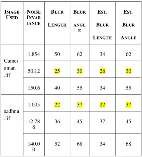
Table 1. Estimated blur angle and blur length with noise
IMAGE
USED
NOISE
INVAR IANCE
BLUR
LENGTH
BLUR
ANGL E
EST.
BLUR
LENGTH
EST.
BLUR
ANGLE
Camer aman .tif
1.854 50 62 34 62
50.12 25 30 26 30
150.6 40 55 34 55
sadhna .tif
1.005 22 37 22 37
12.78 6
36 45 37 45
140.0 0
[image:4.595.56.279.568.676.2]Figure5(a): Real Blurred Figure5(b): Restored Image Image
Table 2. Estimated blur angle and blur length without noise
Figure6: An example of artificially blurred image and corresponding restored images with different restoration technique
Then different images are blurred artificially with different blur angles and lengths. In table 1 column number 2 and 3 shows the blur length and angle used for blurring the images, column number 3 and 4 shows the estimated blurlength and blur angle without noise.
In table 2 column number 2 shows noise variance, column number 3 and 4 shows the detected blurlength and blur angle without noise.
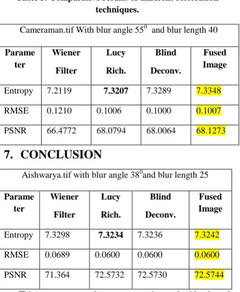
Table3 shows the performance parameters like Entropy, RMSE, PSNR of the restored images for Wiener Filter restoration, Lucy-Richardson Filter and Blind de-convolution filter and the fused image in column no 2, 3, 4, 5 respectively.
IMAGE
USED
BLUR
LENGTH
BLUR
ANGLE
ESTIMATE
LENGTH
ESTIMA TE
BLUR
Cameraman .tif
10
12 11 11
25 37 25 31
45 58 43 58
Sadhna.tif
15 0 8 1
30 45 30 45
Table 3. Comparative results of different restoration techniques.
7.
CONCLUSION
This paper presented process to estimate the blur kernel parameters. The parameters are blur length and blur angle which are used to restore images from the motion blurred images. Different restoration algorithms used to restore the images from motion blurred image has been explained. The comparative results for different restoration methods shows that Lucy Richrdson method gives better result. The experimental results have shown that(i)In artificially blurred images the estimated blur length and blur angle is very close to theoretical value, and (ii) the proposed image restoration techniques effectively restores the images from natural motion blurred, artificial motion blurred and noisy images.(iii)Finally the fused image gives the best results.
8.
REFERENCES
[1] Yogesh K .meghrajani, HimanshuMazumdar, An Interactive Deblurring Technique for Motion Blur,International Journal of Computer Applications (0975 – 8887) Volume 60– No.3, December 2012 . [2] R. Lokhande, K. V. Arya, and P. Gupta. 2006.
Identification of parameters and restoration of motion blurred images. In Proceedings of the 2006 ACM
symposium on Applied computing (SAC '06). ACM, New York, NY, USA, 301-305.
[3] M. M. Chang, A. M. Tekalp, and A. T. Erdem. Blur identification using the bispectrum. IEEE Trans.Signal Processing, 39(10):2323{2325, 1991.
[4] R. Fabian and D. Malah. Robust identification ofmotion and out-of-focus blur parameters from blurredand noisy images. CVGIP: Graphical, Models andImage Processing, 53:403{412, 1991.
[5] HuiJi, Chaoqiang Liu, Motion Blur Identification from Image Gradients, IEEE-978-1-4244-2243-2/08,2008. [6] R. C. Gonzalez and R. E. Woods. Digital
ImageProcessing. Pearson Education, 2003.
[7] D. B. Gennery. Determination of optical transferfunction by inspection of frequency domain plot. J. Opt. Soc. Amer., 63(12):1571{1577, 1973.
[8] Taeg Sang Cho, Blur Kernel Estimation using the Radon Transform, Massachusetts Institute of Technology,2010. [9] Li and Y. Yoshida,‘Parameter estimation andrestoration
for motion blurred images’ IEICE Trans.Fundamentals, E80-A(8), 1997..
[10] Alex Rav-Acha Shmuel Peleg, School of Computer Science and Engineering, Proceedings of the Fifth IEEE Workshop on Applications of Computer Vision (WACV’00), IEEE--7695-0813-8/00, 2000.
[11] Y. S. Chen and I. S. Choa. An approach to estimatingthe motion parameters for a linear motion blurred image. IEICE Trans. Inf. Syst., E83-D(7):1601{1603,2000. [12] R. L. Lagendijk and J. Biemond. Hand Book of Image
and Vedio Processing, chapter Basic Methods for Image Restoration and Identfication, pages 125{140. Academic Press, 2000.
[13] J. S. Lim. Image restoration by short space spectralsubtraction. IEEE Trans. Acoust. Speech SignalProcess., 28(2):191{197, 1980. .
[14] D. G. Childers. The cepstrum: A guide to processing.Proceedings Of The IEEE, 65(10):1428{1443, 1977.
[15] R. Lokhande, K. V. Arya,Identi_cation of Parameters and Restoration of MotionBlurred Images, SAC'06 April 23-27, 2006, Dijon, France.
[16] I. Rekleitis. Visual motion estimation based on motionblur interpretation. Master's thesis, School ofComputer Science, McGill University, 1995.
[17] M. Cannon. Blind deconvolution of spatially invariant image blurs with phase. IEEE Trans. Acoust. Speech Signal Process., 24(1):56{63, 1976.
Cameraman.tif With blur angle 550 and blur length 40
Parame ter
Wiener
Filter
Lucy
Rich.
Blind
Deconv.
Fused Image
Entropy 7.2119 7.3207 7.3289 7.3348 RMSE 0.1210 0.1006 0.1000 0.1007 PSNR 66.4772 68.0794 68.0064 68.1273
Aishwarya.tif with blur angle 380and blur length 25 Parame
ter
Wiener
Filter
Lucy
Rich.
Blind
Deconv.
Fused Image
Entropy 7.3298 7.3234 7.3236 7.3242 RMSE 0.0689 0.0600 0.0600 0.0600 PSNR 71.364 72.5732 72.5730 72.5744