Image Enhancement using Edge Sharpening and
Bidirectional Smooth Histogram Stretching
Umesh Patil
M.Tech Student Oriental College of Technology
Bhopal, India
Kirtee Shevade
Asst. Professor
Oriental College of Technology Bhopal, India
Rajneesh Raikwar
Trainee
Testing campus vijaynagar Bangalore, India
ABSTRACT
This paper introduces two hybrid image enhancement methods “Weighted of Local and Bidirectional Smooth Histogram Stretching” (WLBSHS) and “Local then Bidirectional Smooth Histogram Stretching” (LBSHS). Both methods are almost same and based on local and global enhancement. WLBSHS utilizing local and global enhancement in weighted manner, while LBSHS utilizing them in one by one manner. Local enhancement is achieved based on local standard deviation. Main purpose of local enhancement is sharpening edges of object and exploring local details. For global enhancement this proposed a technique, “Bidirectional Smooth Histogram Stretching” (BSHS). Under BSHS this break histogram in two parts and apply modify forward and backward gamma transform on these parts, with consecutive bin interval control mechanism. Subjective and objective assessments have shown the superiority of our proposed method over existing methods.
Index Terms
local standard deviation (LSD), histogram partition, gamma transform, bidirectional histogram stretching,
I.INTRODUCTION
During last two decades utilization of images in various field such as medical, consumer electronic application, and print media widely increases. This accelerating the research in digital image processing field. To get a high quality visual result, image enhancement techniques are utilized. The main purpose of image enhancement is to bring out hidden details in an image, or to increase the contrast so that image subjectively looks better than the original image [1]. In contrast enhancement changing the pixel‟s intensity of the input image to utilize maximum possible bins [2]. Basically image enhancement is divided into two category, local enhancement and global enhancement. Adaptive contrast enhancement (ACE) [3]-[6] are local enhancement methods. ACE algorithms map the gray values of pixels using the calculation obtained from the local histograms. It utilizes unsharp masking techniques to improve image contrast. Under unsharp masking, image is separated into two components; the low-frequency unsharp mask obtained by low-pass filtering of the image, and the high-frequency component obtained by subtracting the unsharp mask from the original image itself. The high-frequency component is then amplified and added back to the unsharp mask to form an enhanced image. Local enhancement based algorithms only equalize pixels in the finite region, but effectively reduce the impact of other regions, and greatly enhance the local details. In this paper our main concentration on global enhancement. So this briefly describe some global enhancement methods.
Kim [7] proposed a technique, known as “brightness preserving bi-histogram equalization” (BBHE). In this technique image histogram is divided into two sub histogram based, on average intensity. Both sub histograms equalized independently and then merged. The resultant image mean brightness lie between input mean and the middle gray level.
After that, “dualistic sub-image histogram equalization” (DSIHE) has been proposed by Wan et al [8]. The method is same as BBHE except that, histogram is divided based on median value.
Chen and Ramli proposed a scheme called as “recursive mean-separate histogram equalization” (RMSHE) [9]. This technique is a recursive version of BBHE. This technique separates the histogram into two parts based on the mean input brightness. Again these parts further divided based on their respected mean brightness. If
there is r iteration then that will generate 2r histogram pieces. At last
each piece independently equalized and then merged. Result is output image contain mean brightness close to input mean brightness.
Ibrahim and Kong suggest a method “Brightness Preserving Dynamic Histogram Equalization for Image Contrast Enhancement” (BPDHE) [2]. In which enhanced method is achieved by modifying image histogram. This method is actually an extension of MPHEBP [10] and DHE [11]. In BPDHE first Smooth the histogram with Gaussian filter. Then detect the location of local maximums from the smoothed histogram. For each partition new dynamic range is calculated. On the basis of these new dynamic range each partition are equalized independently. And at last normalize the image brightness. Ibrahim and Kong also suggest a method “Color Image Enhancement Using Brightness Preserving Dynamic Histogram Equalization” in which BPDHE utilized for colour images [12].
Above describe methods [7]-[11] only concentrate on mean brightness value. Although image having less mean brightness error, no guarantee to produces natural look and high contrast. Except method [2], [12] all methods based on gray level images, no guideline available to how they utilized for color images.
He et al propose a method “Adjustable Weighting Image Contrast Enhancement Algorithm and Its Implementation” [13] in which weighted average of histogram equalization, exponential transformation and also input image histogram are combined and achieved contrast enhancement. In this method level of the contrast improvement is adjusted by changing the weighting coefficients. This is a simple and effective method over histogram enhancement and exponential transformation. But there is no guide line to how should taken weighted coefficient for different types of image. Taking exponential transform on intensity value implies lacking color due to the risen of intensity.
Chiu et al proposed a method “Efficient Contrast Enhancement Using Adaptive Gamma Correction and Cumulative Intensity Distribution” [14] in which image enhancement is achieved by correcting gamma transform. First of all author redistribute probability distribution of luminance channel. Then calculate cumulative probability distribution based on modified probability distribution. And at last perform gamma transform based on modified cumulative probability distribution. The main aim of this method to avoid fluctuation phenomena due to fluctuated probability distribution, during contrast enhancement through gamma transform. This method only suitable for dimmed images, not applicable for blur lighting images and washout type images, because it stretches image histogram only in forward direction.
After that, take cdf of user interested intensity interval and, cdf of all intensities. Based on these three cdf, drive a virtual histogram. Applying smoothing procedure on virtual histogram in such a manner so that, two consecutive bin does not have difference more than some small constant 2 or 3. Finally apply boundary limiting mechanism to avoiding spikes at the tail end.
VHA work on luminance channel so that it does not maintain color fidelity of image. Edges in image not sharpen as like in point operation based method. Significant artifacts are generated by this method whenever a light source present in the image.
In this paper propose two image enhancement methods “Thisighted of Local and Bidirectional Smooth Histogram Stretching” (WLBSHS) and “Local then Bidirectional Smooth Histogram Stretching” (LBSHS). Both methods not only enhancing global contrast also, sharpen edges, local details and, fully maintaining colour fidelity of image. Under WLBSHS method take weighted result of local and global enhancement. While in LBSHS first perform local enhancement on input image to get locally enhanced image. Then perform global enhancement on this locally enhanced image to get final result. WLBSHS enhancing image in smoothed manner, while LBSHS produce more sharpen edges and local details.
Here carried out “Local Enhancement” (LOCE) sub method for enhancing edges of objects and, local details of image. LOCE is a point operation based method in which utilize sliding window of size 3by3. This window sliding on whole image and, magnifying signals based on local standard deviation. Apply “Bidirectional Smooth Histogram Stretching” (BSHS) for globally enhancing the image. It divides original histogram into two parts based on dividing point. Then left part stretched by applying modify backward gamma transform and, right part is stretched by applying modify forward gamma transform. Each stretched histogram part is smoothed independently and finally merged. LOCE and BSHS both are applying on each colour channel of image independently.
This paper is organized as follows. Section II describes the proposed LBSHS, WLBSHS methods in detail. Section III gives experimental results, and section IV concludes the paper.
II. PROPOSED METHOD
In this section propose two sub methods first is Local Enhancement for exploring local feature of image. And second one is “Bidirectional Smooth Histogram Stretching” for global enhancement of image. Combine result of both sub procedure by two ways. One is combining in weighted manner to get “Weighted of local and Bidirectional Smooth Histogram Stretching” (WLBSHS). And other one is first perform Local Enhancement on original image to get locally enhanced image. In second step Perform BSHS on locally enhance image to get “Local then Bidirectional Smooth Histogram Stretching” (LBSHS). Both WLBSHS and LBSHS are useful for different scenarios.
A.
Local Enhancement
Under local enhancement, calculate the local feature of image. Let x(i, j) represents a pixel value of image. The local area is defined as a (2n+1)×(2n+1) window centered at (i, j). Where n is an odd number. The local mean, i.e. the low-frequency component, of a pixel (i, j) can be computed as
mx=
1
2n + 1 2 x k, l
j+n
l=j−n i+n
k=i−n
(1)
And the local variance calculated as
σx=(2n + 1)1 2 [x k, l − mx(i, j)]2
j+n
l=j−n i+n
k=i−n
(2)
Let f(i, j) denote the enhanced value of x(i, j) then.
f(i, j) = x(i, j) + ( x(i, j) − mx) )
σx
max σx
(3)
Or in compact form
f i, j = L x i, j (4) Here L(.) denote local transformation
B.
Bidirectional Smooth Histogram Stretching
(BSHS)
In this procedure achieve global enhancement. Because the
G channel is a good estimate of the luminance signal [12] so show G
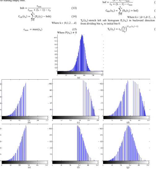
channel histogram under different stages of BSHS procedure in Figure 1. Steps regarding BSHS are as follows
(1) First find a dividing point rd in histogram from which one can
divide the histogram into two parts.
(2) Left part of histogram PL rk is from starting point of histogram
up to dividing point of histogram.
(3) Right part of histogram PR rk started just after from dividing
point to end point of histogram (dividing point is excluded).
(4) Calculate biased cumulative density function CLB rk and
CRB rk for left and right histograms respectively. These
functions are used to construct modify backward gamma transform and, modify forward gamma transform respectively.
(5) For stretching Left part of histogram PL rk utilize modify
backward gamma transform. It stretches histogram towards
backward direction i.e. from dividing point rd to start bin 0.
(6) For stretching Right part of histogram PR rk utilize modify
forward gamma transform. It stretches histogram towards
forward direction i.e. from dividing point rd to last end L-1 bin.
(7) Apply smoothing procedure separately on each histogram.
(8) Combine both histograms to generate modified starched
histogram.
(9) Remap original image pixels value according to modified
histogram to get globally enhanced image.
Let rkє [0, L −1] be the k‟th intensity level, and then the probability
density function (PDF) P(rk) is defined as
P rk =
nk
n 5 for k = 0,1,….. ,L −1
Where nk represents the number of occurrences of rk , and n the total
number of samples in the input image. Here P rk is called the
histogram of the input image. Based on the theory of probability, the cumulative density function (CDF) is defined as
C rk = P rj
k
j=0
6
for k = 0,1,2,…L-1. Note that C(rL−1) =1 by definition. Let m denote mean of intensity
value of image x(i, j). Where i & j are pixel coordinates and r0= 0,
rL−1= L − 1. m є {r0, r1 , r2,… rL−1} where
r0<r1< r2,… rL−2< rL−1. And rdє {r0, r1, r2, … rL−1} is dividing bin
from, which histogram of image i.e. P(rk) is decomposed into two sub
histogram left sub histogram PL(rk) for k=0,1,2,…d and right sub
histogram PR(rk) for k=d+1, d+2 …L-1.
Here dividing bin rd is calculated as
rd= arg minrkabs C rk −
m
L − 1 (7) By definition
PL rk ∪ PR rk = P(rk) (8)
PL rk ∩ PR rk =ϕ (9)
CL rk = PL(rj) k
j=0
(10)
Where k є {0,1,2….d}
CR rk = PR rj k
j=0
11
Where k є {d+1,d+2,….L-1}
Where P(rk) ≠ 0
Here bsb is a bias value proportional to number of empty bin before histogram. This bias is useful to more stretch the left part of histogram over starting empty bins.
bsb = rmin
rmin+ (L − 1) − rd (13)
CLB rk = (PL(rj) k j=0 − bsb) (14)
Where k є {0,1,2….d} rmax = max(rk) (15)
Where P(rk) ≠ 0 Here bsf is a bias value proportional to number of empty bin after histogram. This bias is useful to more stretch the right part of histogram over ending empty bins. bsf = (L − 1) − rmax rd+ (L − 1) − rmax (16)
CRB rk = (PR(rj) k j=0 + bsf) (17)
Where k є {d+1,d+2,….L-1} Tb rk stretch left sub histogram PL rk in backward direction i.e. from dividing bin rd to initial bin 0. Tb rk = rk rrd k CLB rk −1 (18)
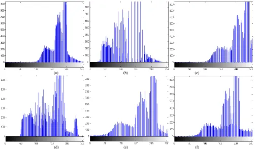
[image:3.595.43.548.106.655.2](a) (b) (c) (d) (e) (f) (g) Figure 1. G-chnal histogram: (a) Original image (b) Modify backward gamma transform on left histogram (c) Modify forward gamma transform on right histogram (d) Combine both histogram after modified gamma transform (e) Smoothed modify backward gamma transform on left histogram (f) Smoothed modify forward gamma transform on right histogram (g) Combine both smoothed left and right histogram. Tf rk stretch right sub histogram PR rk in forward direction i.e. from dividing bin rd to last bin L-1. Tf rk = L − 1 rk L − 1 CRB rk −1 (19)
Tb rk = r0t, r1t, r2t, … … . rdt (20)
Here r0t < r1t < r2t… … . rd−1t < rdt (21)
r0t ≥ 0 (22)
rdt = rd (23)
Tf rk = rd+1t , rd+2t , rd+3t , … … . rL−1t (24)
rd+1t < rd+2t < rd+3t , … … . rL−2t < rL−1t (25)
rd+1t > rdt (26)
rL−1t ≤ L − 1 (27)
34
r0l < r1l < r2l, … … . rd−1l < rdl (29)
r0l ≥ 0 (30)
rdl = rd (31)
ri+1l − ril≤△p (32)
Where i=0,1,2…..d-1 Lt Tf rk = rd+1l , rd+2l , rd+3l , … … . rL−1l (33)
rd+1l , rd+2l , rd+3l , … … . rL−2l < rL−1l (34)
rd+1l = rd+△p (35)
rL−1l ≤ L − 1 (36)
ri+1l − ril≤△p (37)
Where i = (d+1),(d+2),…(L-2) Lt Tb rk ∩ Lt Tf rk = 𝜙 (38)
Lt Tb rk ∪ Lt Tf rk = T rk (39)
Suppose y(i, j) is enhanced image then y i, j = T x i, j (40)
C.
Weighted of Local and BSHS Enhancement
g i, j = w . f i, j + 1 − w . y i, j (41)Where w є [0, 1] g i, j = Mean(x(i, j)) Mean(g(i, j)) g i, j (42
D.
Local Then BSHS Enhancement
h i, j = T L x i, j (43)h i, j = Mean(x(i, j)) Mean(h(i, j)) h i, j (44)
III. RESULT and ANALYSIS
In this section, five image enhancement algorithms are
carried out in our experiments AWICE [13], AGCCID [14]and VHA
[15] and proposed methods „LBDSH‟, „WLBDSH‟. Subjective and Objective assessments both are done on a group of images. Three groups of images are taken and figure 2 to 7 show the results of image enhancement with their green channel histogram for these images. Under Objective assessments five quantitative measurements are utilized to show strength of proposed methods. Table I describe all parameters values taken in our experiment.
A. Subjective assessments
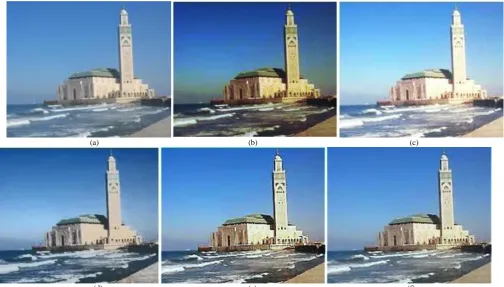
As show in figure2 AWICE increase the contrast but not preserve natural look of image. AGCCID over exposes the image and bluer local details such as windows, doors of building. VHA increase background contrast of image but still lose details of building. Front wall is locking flat and it bluer sea waves. LBDSH and WLBDSH both enhancing contrast with preserving natural visibility of image. Windows, walls texture, doors, boundary, and sea waves all local details clearly enhanced in both images. LBDSH enhance local details in little bit highlighted manner and WLBDSH enhance local details in smother manner.
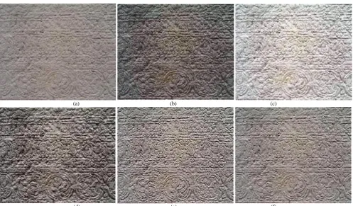
Another simulation results show in figure4 AWICE not preserving natural color combination of image see in middle and boundary area. Although in first view image show rich details, but actually it wider spots, holes, and lines rather than sharpening. AGCCID over enhances the image and it not visually pleasing. VHA little bit succeed to preserving color of image, but instead of sharpening the details it wider dark holes and lines. LBDSH, WLBDSH both sharpening details with preserving natural look of image. Here LBDSH sharpening details in more contrasted manner.
(a) (b) (c)
[image:4.595.43.548.421.708.2](d) (e) (f)
35 (a) (b) (c)
[image:5.595.51.550.67.358.2](d) (e) (f)
Figure 3. G-chnal histogram of image: Historical Building: (a) Original image, (b) AWICE, (c) AGCCID, (d) VHA, (e) LBDSH, (f) WLBDSH
(a) (b) (c)
(d) (e) (f)
[image:5.595.51.549.389.680.2]36 (a) (b) (c)
[image:6.595.49.555.68.358.2](d) (e) (f)
Figure 5. G-chnal histogram of image: Wall: (a) Original image, (b) AWICE, (c) AGCCID, (d) VHA, (e) LBDSH, (f) WLBDSH
(a) (b) (c)
(d) (e) (f)
[image:6.595.50.550.381.671.2]37 (a) (b) (c)
(d) (e) (f)
Figure 7. G-chnal histogram of image: Statue: (a) Original image, (b) AWICE, (c) AGCCID, (d) VHA, (e) LBDSH, (f) WLBDSH
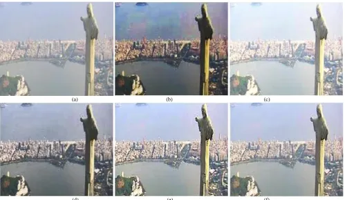
In figure6 AWICE introduced extra red color and checks in sky. It increased unwanted artifacts surrounding statue and darken middle portion of statue. AGCCID increases only mean brightness rather than contrast. VHA little bit succeed to increase the contrast but darken the statue and ponds water and blurring upper portion of far city buildings. LBDSH increase the contrast with sharpening details such as statue, side hill, cloud in sky, reflection of building in pond and also far buildings in very clear manner. These entire objects are also having good visibility in image enhanced by WLBDSH with preserving natural look of image. By simulation result can easily see LBDSH and WLBDSH both enhancing the image. LBDSH is specially used whenever want extra attention on local details, such as in wash out type image or a too bluer image. And WLBDSH is used in normal case.
Preserving the overall shape of histogram, corresponding to their bins and smoothness of histogram is responsible for natural look of image. And also utilization of more bins by image histogram showing good enhancement of image. By observing figure 3, 5, 7 AWICE although utilize almost all bins but it not preserving the histogram shape with their respective bins. It also shows zigzag nature. AGCCID compress histogram at higher bins and not utilizing starting bins. VHA also not utilize full bins except figure 5 (d). Due to more zigzag nature some time it over expose small details. In figure 2(d) it looks like three doors in left wall but only middle door is real. LBDSH and WLBDSH both are, utilizing all bins with preserving shape, smoothness and symmetry of histogram in all cases.
B. Objective assessments
Here done objective quality assessments based on five parameter Absolute Mean Brightness Error (AMBE) [16],[17], Discrete Entropy (E) [18]-[21], Peak Signal-to Noise Ratio (PSNR)
[17], Measure of Enhancement (EME) [21]-[24] and Brenner‟s
measure (BR) [24], [25].
By observing Table II to IV can see that LBDSH always generate very high value of EME and BR compare to all methods. And lowest AMBE value compares to first three methods AWIE, AGCCID, VHA. It also shows high range value of E and PSNR.
WLBDSH always generate lowest AMBE value compare to all methods. In almost all cases it show highest PSNR value and high range value of E and EME. Although in table II and IV VHA show higher value of E, but it‟s doesn‟t mean that our methods inferior in case of rich detail. As clearly show in figure 2 VHA vanished middle and lower window of minaret (tower) and in figure 3 images loses natural looks. On the other hand LBDSH, WLBDSH both enhances the image details, with preserving natural look.
Common assumption for expression (45) to (50) M≔ Number of pixel row in image
N≔ Number of pixel column in image MN≔ Total number of pixel in image Ii i, j ≔ (i, j)‟th pixel value of input image
Io i, j ≔ (i, j)th pixel value of output image
[image:7.595.48.551.69.362.2]I i, j ≔ (i, j)th pixel value of image L-1≔ Maximum possible pixel value
TABLE I Parameters used for all method
Method\Parameter Weighted Parameter Window Size Maximum bin interval Other Parameter
AWIE қ=3, λ=1 _ _ ε=0.009
AGCID _ _ _ _
VHA w=2, v=2 3×3 t=2 Pk10=16, Pk1=40, Tla=3
LBDSH w=0.5 3×3 △p=2 _
38 TABLE II Performance for image Historical Building
Method\Criteria AMBE E PSNR EME BRE
Original 0 7.31172 Inf 26.4991 226.9653
AWIE 39.01437 7.413503 15.36301 31.04844 430.6295
AGCID 39.93584 7.18745 15.43147 27.25027 345.9669
VHA 7.966074 7.618879 20.62694 29.79152 470.4593
LBDSH 0.242519 7.465714 18.7271 60.37881 1359.592
WLBDSH 0.024207 7.536805 24.21313 32.37584 660.9093
TABLE III Performance for image Wall
Method\Criteria AMBE E PSNR EME BRE
Original 0 6.383573 Inf 33.04501 484.1448
AWIE 39.49559 6.970566 15.38121 49.19412 1701.188
AGCID 39.93584 7.18745 15.43147 27.25027 345.9669
VHA 51.46664 7.001415 13.2601 38.48288 1970.932
LBDSH 0.143222 7.596913 15.12926 172.9798 5502.371
WLBDSH 0.016296 7.354528 21.27325 54.36543 2198.006
TABLE IV Performance for image Statue
Method\Criteria AMBE E PSNR EME BR
Original 0 6.774238 Inf 25.75925 360.6179
AWIE 60.94624 7.27337 11.91305 32.02176 993.8139
AGCID 32.75381 6.724087 17.41127 26.31368 549.2485
VHA 36.83814 7.435518 15.43661 30.73465 1195.116
LBDSH 0.747496 7.149142 18.47179 46.94285 2514.084
WLBDSH 0.062296 7.245465 23.49494 31.10103 1212.019
1) AMBE: It is an absolute mean difference between input and output
image brightness. Lower AMBE value indicates that the mean
brightness better preserved.
AMBE = 1
MN Ii i, j
N
j=1 M
i=1
− Io i, j
N
j=1 M
i=1
45
2) E: The discrete entropy is used to measure the content of an image. Generally, the higher value of discrete entropy indicates image is fulfilling with richer details.
E = P rk log2 P rk (46) L−1
k=0
Where rk represent color bin and P(rk) is normalize count pixels
having colour rk.
3) PSNR: Here PSNR stands for Peak Signal-to-Noise Ratio. Noise is taken as root mean-squared error (RMSE)
Higher PSNRvalue represents greater image quality.
PSNR = 20log10
255
RMSE (47) Where RMSE is, defined as
RMSE = 1
MN Ii i, j − Io i, j 2
N
j=1 M
i1
(48)
4) EME: This value is an approximation of the averaged contrast in the image. The EME approximates an average contrast by partitioning
the image into numbers of non-overlapped sub-blocks of size k1 by
k2. And then finding a measure based on ratio of the minimum and
maximum gray values in each sub-block. Finally averages them to
generate the result.Higher EMEvalue represents local details are well
enhanced in image.
EME = M1
k1
N k2
20InMax Iw i,j + con
Min Iw i,j + con
N k2
j=1 M k1
i=1
(49)
Where con is small value for avoiding zero values. Iw i,j is image block of size k1by k2 and (i, j) represents block index. In our
experiment take con=0.0001 and k1=8, k2=8. Max Iw i,j and
Min Iw i,j return maximum and minimum value for block indexed
by (i, j). . Represents floor function.
5) BR: Brenner‟s measure is used for sharpness assessment. Higher value of BR indicates more sharpness of image.
BR = I i, j − I i + 2, j 2
N
j=1 M−2
i=1
(50)
IV. CONCLUSION
In this paper, we proposed two hybrid approaches those are combination of two sub methods, local enhancement and Global enhancement. Local enhancement achieved through our local standard deviation based formula. Global enhancement achieved by smoothly stretching histogram in both directions using modified gamma transform. And finally combine them weighted manner and one by one manner in WLBDSH and LBDSH respectively. The experimental
result based on subjective assessments and objective assessments
39
V. REFERENCES
[1] Rafael C. Gonzalez, and Richard E. Woods, Digital Image
Processing, 2nd edition, Prentice-Hall of India: New Delhi, 2002.
[2] H. Ibrahim, and N.S.P. Kong, “Brightness preserving dynamic
histogram equalization for image contrast enhancement,” IEEE
Transactions on Consumer Electronics, vol. 53, no. 4, pp. 1752-1758, Nov. 2007.
[3] G. Deng, L. W. Cahill, and G. R. Tobin, “The study of logarithmic
image processing model and its application to image
enhancement,” IEEE Trans. Image Processing, vol. 4, pp. 506–
512, Apr. 1995.
[4] T. L. Ji, M. K. Sundareshan, and H. Roehrig, “Adaptive image
contrast enhancement based on human visual properties,” IEEE
Trans. Med. Imag. Proc., vol. 13, pp. 573–586, Aug. 1994.
[5] Kentaro Kokufuta and Tsutomu Maruyama, “Real-time processing
of local contrast enhancement on FPGA.” In International
conference on field programmable logic and applications, Prague, pp. 288-293, 2009.
[6] J. Alex Stark, “Adaptive image contrast enhancement using
generalizations of histogram equalization.” IEEE Trans. Imag.
Proc., vol.9, No.5, pp. 889-896, May. 2000.
[7] Yu Wan, Qian Chen and Bao-Min Zhang, “Image enhancement
based on equal area dualistic sub-image histogram equalization
method”, IEEE Trans. Consumer Electron., vol. 45, no. 1, pp.
68-75, Feb. 1999.
[8] Soong-Der Chen, and Abd. Rahman Ramli, “Minimum mean
brightness error bi-histogram equalization in contrast
enhancement”, IEEE Trans. Consumer Electron., vol. 49, no. 4,
pp. 1310-1319, Nov. 2003.
[9] Soong-Der Chen, and Abd. Rahman Ramli, “Contrast
enhancement using recursive mean-separate histogram
equalization for scalable brightness preservation”, IEEE Trans.
Consumer Electron., vol. 49, no. 4, pp. 1301-1309, Nov. 2003.
[10]K. Wongsritong, K. Kittayaruasiriwat, F. Cheevasuvit, K. Dejhan,
and A. Somboonkaew, “Contrast enhancement using multipeak
histogram equalization with brightness preserving”, IEEE
Asia-Pacific Conference on Circuit and System, pp. 455-458, 24-27 Nov. 1998.
[11]M. Abdullah-Al-Wadud, Md. Hasanul Kabir, M. Ali Akber
Dewan, and Oksam Chae, “A dynamic histogram equalization for
image contrast enhancement” IEEE Trans. Consumer Electron.,
vol. 53, no. 2, pp. 593-600, May 2007.
[12]Nicholas Sia Pik Kong, and Haidi Ibrahim, “Color Image
Enhancement Using Brightness Preserving Dynamic Histogram
Equalization” IEEE Transactions on Consumer Electronics, Vol.
54, No. 4, pp.1962-1968, Nov. 2008.
[13]Renjie He, Sheng Luo, Zhanrong Jing, Yangyu Fan, “Adjustable
Weighting Image Contrast Enhancement Algorithm and Its
Implementation” IEEE Conference on Industrial Electronics and
Applications, pp.1750-1754, June 2011.
[14] Yi-Sheng Chiu, Fan-Chieh Cheng and Shih-Chia Huang, “Efficient
Contrast Enhancement Using Adaptive Gamma Correction and
Cumulative Intensity Distribution” IEEE International Conference
on Systems, Man, and Cybernetics (SMC), pp. 2946 -2950, 9-12 Oct. 2011.
[15] Zhengya Xu, Hong Ren Wu, Xinghuo Yu, “Colour Image
Enhancement by Virtual Histogram Approach” IEEE Transactions
on Consumer Electronics, Vol. 56, No. 2, May 2010.
[16] M. Kim and M. G. Chung, “Recursively separated and weighted
histogram equalization for brightness preservation and contrast
enhancement” IEEE Trans. Consumer Electron., vol. 54, no. 3,
pp.1389–1397, Aug. 2008.
[17] Pei-Chen Wu, Fan-Chieh Cheng, Yu-Kumg Chen, “A Weighting
Mean-Separated Sub-Histogram Equalization for Contrast
Enhancement” International Conference on Biomedical
Engineering and Computer Science (ICBECS), pp. 1-4, 23-25 April 2010.
[18] Tarik Arici, Salih Dikbas and Yucel Altunbasak, “A histogram
modification framework and its application for image contrast
enhancement.” IEEE Trans. Imag. Proc., vol.18, No.9, pp.
1921-1935, Sep. 2009.
[19] Ying Shan, Hua Ye and Guang Deng, “A successive mean splitting
algorithm for contrast enhancement and dynamic rang reduction.” International Symposium on Communications and Information Technologies(ISCIT), Sydney, pp. 753-758, 2007.
[20] A.Beghdadi and A.L.Negrate, “Contrast enhancement technique
based on local detection of edge.” Comput. Vis, Graph., Image
Process, vol.46, No.2, pp. 162-174, May. 1989.
[21] Bin Liu, Weiqi Jin, Yan Chen, Chongliang Liu, and Li Li,
“Contrast Enhancement using Non-overlapped Sub-blocks and
Local Histogram Projection” IEEE Transactions on Consumer
Electronics, Vol. 57, No. 2, pp. 583 – 588,May 2011.
[22] Sos.S.Agaian, Karen A. Panetta and A. Grigoryan,
“Transform-based image enhancement algorithms with performance measure.” IEEE Trans. Imag. Proc., vol.10, No.3, pp. 367-382, Mar. 2001.
[23] Sos.S.Agaian, Blair Silver and Karen A. Panetta, “Transform
coefficient histogram-based image enhancement algorithms using
contrast entropy.” IEEE Trans. Imag. Proc., vol.16, No.3, pp.
741-758, Mar. 2007.
[24] Tzu-Cheng Jen and Sheng-Jyh Wang, “Bayesian
Structure-Preserving Image Contrast Enhancement and Its Simplification” IEEE Trans. on Circuits and Systems for Video Technology, vol.16, No.6, pp. 831-843, June 2012.
[25] Ming-Suen Shyu and Jin-Jang Leou, “A genetic algorithm
approach to color image enhancement,” Pattern Recognition, Vol.