Munich Personal RePEc Archive
Relationships among Household Saving,
Public Saving, Corporate Saving and
Economic Growth in India
Sinha, Dipendra and Sinha, Tapen
Ritsumeikan Asia Pacific University, Japan and Macquarie
University, Australia and ITAM, Mexico
21 February 2007
Online at
https://mpra.ub.uni-muenchen.de/2597/
RELATIONSHIPS AMONG HOUSEHOLD SAVING, PUBLIC SAVING, CORPORATE SAVING AND ECONOMIC GROWTH IN INDIA
Corresponding author:
Dipendra Sinha, Ritsumeikan Asia Pacific University, Japan and Macquarie University, Australia, E-mail: [email protected]
[email protected] Address: Ritsumeikan Asia Pacific University Beppu, Oita 874-8577
JAPAN
Phone: +81-977-78-1214 Fax: +81-977-78-1123
Tapen Sinha, Instituto Tecnologico Autonomo de Mexico (ITAM), Mexico E-mail: [email protected]
Abstract:
This paper examines the relationship between the growth rates of household saving, public saving, corporate saving and economic growth in India using multivariate Granger causality tests. The conventional wisdom suggests that the causality flows from saving to economic growth. We show that the causality goes in the opposite direction for India. Hence, higher saving is the consequence of higher economic growth and not a cause.
JEL Codes: E21, O11, O16
1. Introduction
After fifteen years of economic reforms, India has finally embarked on a growth path
never seen before in the history of the subcontinent. This has led to a resurgence of
interest on economic growth in India. A number of popular magazines have picked up on
this theme. In a recent article, the Economist (2006) declared: “…it is argued, will help
raise the level of private savings from about 29% of GDP now to 34% over the next five
to seven years. Investment will follow, so GDP will continue to grow at 8%”. Clearly, the
presumption is that the growth in saving now will lead to a growth in GDP in the future.
In theories of economic growth such as that of Solow (1956), higher economic growth
follows from higher saving. This has been the conventional wisdom. The World Bank
regularly recommends developing countries to adopt policies that increase the saving rate
for these countries to achieve a higher rate of economic growth.
Recently, a number of studies have examined the relationship between saving and
economic growth. Our study provides the following new elements to uncover saving and
economic growth relationship in India. First, we use three distinct measures of saving:
household saving, public saving and corporate saving. Second, we conduct multivariate
Granger causality tests to examine the relationship. No other previous studies have used
2. Previous Studies
A number of studies examine the relationship between saving and economic growth.
Using annual data for India, Sinha (1996) looks at the causality between the growth rates
of gross domestic saving and gross domestic private saving and economic growth. The
bivariate causality results show that there is no causality running in either direction
between the growth rate of gross domestic private saving and economic growth or
between the growth rate of gross domestic saving and economic growth. Sinha and Sinha
(1998) perform multivariate causality tests between the growth rates of private saving and
public saving and economic growth for Mexico. The results show that the growth rates of
private and public saving Granger cause economic growth. However, there is no evidence
of reverse causality. This runs counter to the conventional wisdom. For Pakistan, Sinha
(1998-1999) finds somewhat different results. Using annual data for 1960-1995 and an
augmented Granger causality tests in an error-correction framework, he finds that growth
rate of GDP Granger causes the growth rates of both private saving and total saving.
However, the growth rate of private saving is found not to be Granger causing growth of
GDP while the growth of total saving is found to be causing the growth of GDP. Sinha
(2000) finds similar results for the Philippines.
While the above studies find evidence mostly contradictory to the conventional wisdom,
Sinha (1999) finds some evidence that causality flows from both gross domestic saving
and from gross domestic private saving to economic growth for Sri Lanka. So, the
find support for the conventional wisdom for Mexico when foreign direct investment is
taken into account as a form of foreign saving.
3. The Present Study
We use two data sources. These are the Economic Survey of India (2006) and the
International Financial Statistics of the International Monetary Fund (2006). We
collected annual data for 1950-2001 for GDP, household saving, public saving and
corporate saving. All data are in billions of Indian rupees and are in real terms
(2000=100). We construct growth rates of each variable. Specifically, we examine the
relationships among growth rates of the GDP (denoted by GDPGR), household saving
(denoted by HHSAVGR), public saving (denoted by PUBSAVGR) and corporate saving
(denoted by CORPSAVGR) respectively. The causality tests are valid if the variables are
either stationary or cointegrated. Therefore, we examine the stationarity of each variable.
We use the Kwiatkowski-Phillips-Schmidt-Shin (1992)for testing for stationarity. The
test takes trend or level stationarity as the null hypothesis. In contrast, the augmented
Dickey-Fuller and Phillips-Perron tests take the unit root as the null hypothesis.
Let us consider the following equation consisting of a deterministic trend, random walk
and stationary error:
where νt is a stationary process, t is the time trend and ct follows the random walk ct = ct-1
+ µt with µt ~ iid(0, σ2µ). The null hypothesis is: σ2µ = 0 or ct is a constant. We can drop
the trend term in (1) if we want to test the stationarity of a non-trend variable.
As Maddala and Kim (1998) point out, equation (1) is a special case of a test for
parameter constancy against the alternative that parameters follow a random walk. This
was first considered by Nabeya and Tanaka (1988). In Nebaya and Tanaka, the test
statistic is as follows:
LM = 2 ˆ 1 2 e T t St
σ
∑ = (2)
In (2), et are the residuals from the regression of yt on a constant and time trend. is the
residual sum of squares divided by T (or residual variance) and S
2 ˆe σ
t = where t =
1,2,…..T. This is an upper tail test. When errors are not iid, the appropriate denominator
of (2) is an estimator of σ
∑ = T i i e 1 2
that Kwiatkowski-Phillips-Schmidt-Shin interpret as the “long
run variance,” rather than of σˆe2. σ2 equals lim T 1E(ST2). A consistent estimator of σ
T
− ∞ →
2
is given by
∑ = =∑+ − − + ∑ = − = l s T s t t s
e t e l s T T t t e T l s 1 1 ) , ( 1 2 1 2 1 ) (
) , (s l
ω is an optional lag window that corresponds to the choice of a spectral window.
Kwiatkowski-Phillips-Schmidt-Shin use the Bartlett window,
1 1 ) , ( + − = l s l s
ω . This
ensures the non-negativity of . The lag parameter is set to correct for residual serial
correlation. If the residuals are iid, then a lag of zero is appropriate. All variables in our
study, namely, GDPGR, HHSAVGR, PUBSAVGR and CORPSAVGR are found not to
have trends. The results of the Kwiatkowski-Phillips-Schmidt-Shin unit root test are
displayed in Table 1. The results show that none of the variables has a unit root. Thus, we
employ the block Granger non-causality tests (Granger, 1969).
) ( 2 l
s l
The methodology for the block Granger causality is as follows. Consider the augmented
vector autoregressive model:
zt = a0 + a1t + φ
i p
=
∑
1
i zt-i + Ψwt + ut (4)
where zt is an m x 1 vector of jointly determined (endogenous) variables, t is a linear time
trend, wt is q x 1 vector of exogenous variables, and ut is an m x 1 vector of unobserved
disturbances. Let zt = (z/1t, z/2t)/, where z/1t and z/2t are
m1 x 1 and m2 x 1 subsets of zt, and m = m1 + m2. We can now have the block
decomposition of (3) as follows:
z1t = a10 + a11t + φ
i p
=
∑
1
i, 11 z1,t-i + φ
i p
=
∑
1
z2t = a20 + a21t + φ
i p
=
∑
1
i, 21 z1,t-i + φ
i p
=
∑
1
i, 22 z2,t-i + Ψ2wt + u2t (6)
The hypothesis that the subset z2t do not ‘Granger cause’ z1t is given by
HG: φ12 = 0 where φ12 = (φ1,12, φ2,12 . . ., φ1p,12).
4. Results
Table 1 gives the results of unit root tests. The results show there are no unit roots in our
series of four variables. Therefore, Granger causality does not produce spurious
correlations. If some of the variables did exhibit unit roots, we could not be sure that
standard causality tests are not the results of such data generating processes.
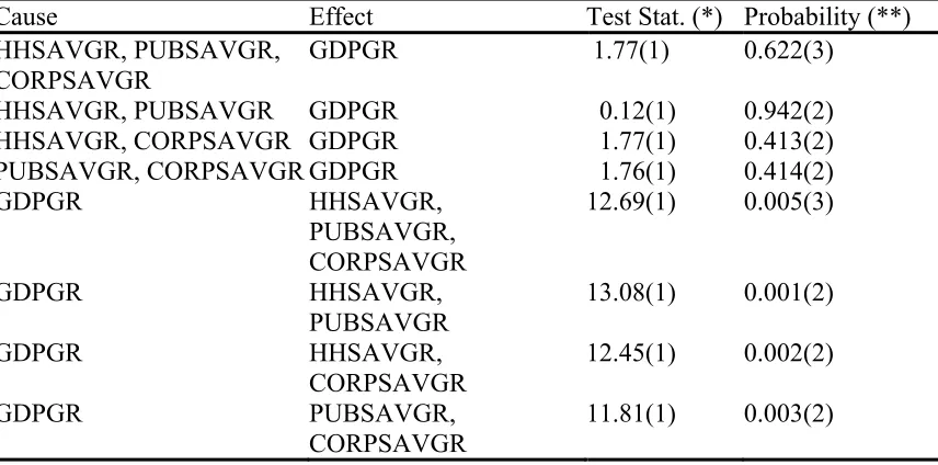
Table 2 provides the results of a series of (block) causality tests postulated in equations (5)
and (6) above. We asked tested two sets of causalities. First, we test to see if the growth
rate in GDP is caused by (in the Granger sense) one or more of different components of
total saving in India. Any number of combinations point to the same inevitable
conclusion: there is no causality flowing from different components of saving to the
growth rate of GDP. Second, we test to see if various combinations of different
components of total saving is caused by the growth rate of GDP. The answer is inevitably
positive. Thus, economic growth is Granger causally prior to household saving, corporate
5. Conclusion
We showed that in India, over a period of five decades, economic growth has produced
higher saving in various forms and never the other way around. The policy implication is
References
Alguacil M, Cuadros A and Orts V. 2004. Does saving really matter for growth? Mexico (1970-2000). Journal of International Development 16(2): 281-290.
Economic Survey of India.2006. (http://indiabudget.nic.in/es2005-06/esmain.htm)
The Economist. 2006. Business in India: Can India fly? Print Edition, June 1 (Special Section).
Granger CWJ. 1969. Investigating causal relations by econometric models and cross spectral methods. Econometrica 37(3):424-438.
International Monetary Fund. 2006. International Financial Statistics, Online version, July.
Kwiatkowski D, Phillips PCB, Schmidt P and Shin Y. 1992. Testing the null hypothesis of stationarity against the alternative of a unit root: How sure are we that economic time series have a unit root? Journal of Econometrics 54(1-3):159-178.
Nabeya S, Tanaka K. 1988. Asymptotic theory of a test for the constancy of regression coefficients against the random walk alternative. Annals of Statistics 16(1):218-235.
Sinha D. 1996. Saving and economic growth in India. Economia Internazionale 49(4): 37-647.
Sinha D, Sinha T. 1998. Cart before the horse? The saving-growth nexus in Mexico.
Economics Letters 61(1):43-47.
Sinha D. 1998-1999. The role of saving in Pakistan’s economic growth. Journal of Applied Business Research 15(1), 79-85.
Sinha D. 1999. Saving and economic growth in Sri Lanka. Indian Journal of Applied Economics 8(3):163-174.
Sinha D. 2000. Tests of Granger causality between saving and economic growth in the Philippines. Journal of Social and Economic Development 3(3): 200-207.
Table 1. Kwiatkowski-Phillips-Schmidt-Shin Unit Root Tests (No Trends) Variable Test Statistic
GDPGR 0.2770 HHSAVGR 0.3809 PUBSAVGR 0.1113 CORPSAVGR 0.1238
Table 2. Multivariate Granger Causality Tests
Cause Effect Test Stat. (*) Probability (**) HHSAVGR, PUBSAVGR,
CORPSAVGR
GDPGR 1.77(1) 0.622(3)
HHSAVGR, PUBSAVGR GDPGR 0.12(1) 0.942(2) HHSAVGR, CORPSAVGR GDPGR 1.77(1) 0.413(2) PUBSAVGR, CORPSAVGR GDPGR 1.76(1) 0.414(2) GDPGR HHSAVGR,
PUBSAVGR, CORPSAVGR
12.69(1) 0.005(3)
GDPGR HHSAVGR, PUBSAVGR
13.08(1) 0.001(2)
GDPGR HHSAVGR, CORPSAVGR
12.45(1) 0.002(2)
GDPGR PUBSAVGR, CORPSAVGR
11.81(1) 0.003(2)