Object Recognition using Disk based Morphological
Shape Decomposition Features
G. Rama Mohan Babu
Assoc. Prof., Dept. of I.T.,RVR & JC College of Engineering, Guntur, INDIA
B. Raveendra
Babu,
Ph.DProfessor, Dept. of CSE VNR VJ Institute of Engg. and Technology,
Hyderabad, INDIA
A. Srikrishna,
Ph.DProfessor, Dept. of IT, RVR & JC College of
Engineering, Guntur, INDIA
N. Venkateswara Rao
Assoc. Porf., Dept. of CSERVR & JC College of Engineering, Guntur, INDIA
A
BSTRACTThe ability of object recognition system is to recognize a large number of objects constrained by a variety of factors such as the selection of a feature extraction method, quality of the images, and the classification models. This paper presents an approach to the recognition of complex shape objects using shape representation features. The shape representation features are the disk components which are calculated from morphological shape decomposition technique. The disk components of the shapes are generated using disk component generation Algorithm. These disk components are more primitive and easily matched with other disk components that are from another shape. These features are tested using the Quadratic classifier on different shapes. It is observed that the classifier gives good accuracy.
General Terms
Pattern recognition, Machine learning.
Keywords
Mathematical morphology, Shape decomposition, Disk components, Feature vector, Object recognition, and Classification.
1.
INTRODUCTION
Object recognition and classification tasks arise in a very wide variety of practical situations, such as detecting faces from video images, finding tanks and helicopters from satellite images, identifying suspected terrorists from fingerprint images, and diagnosing medical conditions from X-rays [1–5]. In many cases, people (possibly highly trained experts) perform the recognition/classification tasks well, but there is either a shortage of such experts or the high cost in paying the experts. Given the amount of image data containing objects of interest that need to be classified and recognized, automatic computer based classification and recognition programs/systems are of immense social and economic value. A classification or recognition program must correctly map an input vector describing an instance (such as an object image) to one of a small set of class labels. Writing classification or recognition programs that have sufficient accuracy and reliability is usually very difficult and often infeasible: human programmers often cannot identify all the subtle
conditions needed to distinguish between all instances of different classes.
The mathematical morphology is a shape-based approach to image processing [6, 7]. Basic morphological operations can give interpretations using geometric structures in terms of shape, size, and distance. Therefore, mathematical morphology is specially suited for handling shape-related processing and operations. Mathematical morphology also has a well-developed mathematical structure, which facilitates the development and analysis of morphological image processing algorithms. A number of morphological shape representation schemes have been proposed [8–22]. Many of authors use the structural approach, i.e. a given shape is described in terms of its simpler shape components and the relationships among those components.
transform is that it leads to an efficient shape decomposition scheme. In this scheme, a given shape is decomposed into a collection of modestly overlapping octagonal shape components. These octagonal components are more primitive than the components obtained from the MSD or OMSD. Each octagonal component is represented by a single center point and the overlapping level is reduced. The main problem with this decomposition scheme is that the generalized skeleton transformation needs to be applied multiple times. Another problem is that although it is easier to compare two octagons than to compare two shape components from the MSD or OMSD, it is still, not a trivial task to define a meaningful similarity measure for such octagonal components. Then an octagon-fitting algorithm (OFA) [23] was introduced which finds a special maximal octagon for each image point of a given shape. The OFA allows the development of two new shape decomposition algorithms. The first decomposition algorithm will use octagonal shape components. The general decomposition algorithm uses disk components. However, the OFA will only need to be applied once.
In this paper, we present an object recognition algorithm that is based on the morphological shape decomposition algorithm. Recognition is carried out by using shape’s disk components. These disk components are matched basing on both geometrical and structural information extracted from the structural representations. The recognition is simple and easy with these shape disk components. The organization of the paper is as follows.
Section 2 describes the overall methodology for classification and recognition. Section 3 shows experimental results and discussions, and the conclusions are given in Section 4.
2.
M
ETHODOLOGYOur approach to object recognition consists of the training of cascade of classifiers that discriminates object features from the background. The feature is defined as a function of one or more measurements, each of which specifies some experimental property of an object.
Several steps are used to identify the shape components for classification of objects. The technique presented here is to decompose a binary shape into a union of simple binary shape components. The decomposition is unique and invariant to rotation, translation and scaling. The techniques used in the decomposition are based on mathematical morphology [6].
2.1
Generating Disk Components
We assume that our objects are well characterized by their shape properties, and that the shape properties are represented by binary shape components extracted from the image. For this reason, we classify each query by identifying the disk components and various features using these disk components.
For generating disk components, eight structuring elements B0, B1, B2, …, B7 are used as shown in figure 1. We use all the eight structuring elements in order for the final shape elements to be as symmetric as possible. The shape elements are represented by the center of the disk and by the size of the disk. The shape element generated by the basic structuring element for the different sizes is given in figure 2. The disk size 1 (S1) is generated by dilating the center pixel with B0, the disk of size 2 (S2) is generated by the disk
of size 1 (S1) using the B1 structuring element, and the disk of size
3 (S3) is generated by the disk of size 2 (S2) using the B2
structuring element and so on. These disk components are shown in figure 2(a), 2(c), and 2(e) respectively.
The sequence of basic structuring element is recorded in the expression for finding disk sizes. In general, a disk Si of size i is generated by
𝑆
𝑖= 𝑆
𝑖−1⨁𝐵
[image:2.612.320.554.146.343.2]𝑖−1 𝑚𝑜𝑑 8
𝑤ℎ𝑒𝑟𝑒 𝑖 > 0
(1)
Fig. 1: Eight two-point structuring elements.
Fig. 2: Shape elements generated using two-point structuring elements: (a) B0; (b) 𝑩𝟎⊕ 𝑩𝟒; (c) 𝑩𝟎⊕ 𝑩𝟏; (d) 𝑩𝟎⊕ 𝑩𝟏⊕
𝑩𝟓; (e) 𝑩𝟎⊕ 𝑩𝟏⊕ 𝑩𝟐; (f) 𝑩𝟎⊕ 𝑩𝟏⊕ 𝑩𝟐⊕ 𝑩𝟒; (g) 𝑩𝟎⊕ 𝑩𝟏⊕ 𝑩𝟐⊕ 𝑩𝟑.
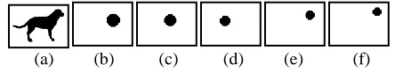
The complete process of generating disk components [25] is given in Algorithm 1. The first five largest disk components are shown in figure 3.
Fig. 3: (a) is the original image; (b) to (f) are the first five largest disk components respectively.
Algorithm 1
Input: Binary Image.
Output: Table D consists of disk components.
1.
ƒ(x, y) ← Preprocessed binary image.2.
Generate disk components for ƒ(x, y) using Disk Generating Algorithm (DGA) [17].3.
The disk size Si, and disk center (xi, yi), and structuring element sequence is stored into a table T.4.
ƒ′(x, y) ← 0.5.
While T is not empty do6.
Vector V ← Delete Maximum size disk from T.7.
If this disk is not present in the image ƒ′(x, y) then append size and center of the disk component into Disk component into table D(Si, xi, yi).
8.
ƒ″(x, y) ← 0 and dilate ƒ″ to vector V using equation (1).9.
ƒ′(x, y) ← ƒ′(x, y) U ƒ″(x, y).10.
End while.
2.2
Feature Extraction
Disk components summarize the local shape in image neighborhoods in terms of the density of pixels in those
(a) (b) (c) (d) (e) (f) 0 0 0 0 0 0 0 1 0 0 0 0 0 0 0 0 0 1 0 0 0 1 0 0 0 1 1 0 1 0 0 1 0 0 1 0 1 1 0 0 1 0 0 1 0 0 1 0 0 0 0 1 0 0 0 0 0 0 0 1 0 0 0 0 0 0 0 1 0 0 0 0
[image:2.612.320.542.391.432.2]neighborhoods. By computing features at a set of image neighborhoods surrounding a query disk, we summarize the overall shape properties of the image, which should be a discriminating recognition cue for our shape-based objects. The features identified using the disk is given in algorithm 2.
Algorithm 2
Input: Disk Components table D.
Output: Feature vector X consists of 7 features.
1.
Nt is the total number of all disk components. i.e. Nt = number of rows of the table D.2.
Sm is the maximum disk size among all disk components.𝑆𝑚 = 𝑀𝐴𝑋(𝐷(𝑆𝑖)) (2)
3.
L is the distance between the first two largest disk components. Let the first largest disk component Sm and the second largest disk component Sn. The centers of these two disk components are (xm, ym) and (xn, yn) respectively from table D, then the distance is𝐿 = (𝑥𝑛− 𝑥𝑚)2+ (𝑦𝑛− 𝑦𝑚)2 (3)
4.
Nd is the total number of distinct disk components i.e. two disk components Si and Sj are distinct components if and only if i≠j.𝑁𝑑= 𝑑𝑖𝑠𝑡𝑖𝑛𝑐𝑡 𝐷(𝑆𝑖) (4)
5.
Sa is the average size of the distinct disk components. It is the ratio between the sum of distinct disk sizes and the number of such disks.𝑆𝑎 = 𝑑𝑖𝑠𝑡𝑖𝑛𝑐𝑡 (𝐷(𝑆𝑖))
𝑁𝑑 (5)
6.
N0 is the total number of isolated pixels or zero size disk components (S0).𝑁0= 𝑐𝑜𝑢𝑛𝑡(𝐷(𝑆0)) (6)
7.
Nr is the number of disk components needed to reconstructthe original shape image f. Note that all disk components are not required to reconstruct the original image.
The seven disk component features are identified to recognize objects characterized by their shape properties. The objects are well characterized by their shape properties, and the shape properties are represented by disk components from the image. The classification performed is based on the values of disk features that summarize the local shape in image neighborhoods in its immediate vicinity.
2.3
Classification
Supervised classification algorithms aims at predicting the class label h ∈ {1, …, l} from among l predetermined classes that correspond to a query x0 composed of m characteristics, i.e., x0 = {x1,…, xm}0 ∈ Rm. To perform this task, a classification scheme c “ascertained” from the training set T = {(xi, ei) : i = 1,…, n} is required.
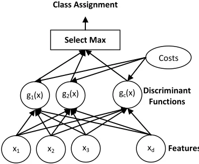
The classifier is said to assign a feature vector x to class wi if gi(x)>gj(x) for all j≠i, where gi(x), i=1, 2, …, c is a discriminant function. Hence the classifier is viewed as a network or machine as shown in figure 4, which computes c discriminant functions and selects the category corresponding to the largest discriminant.
For the minimum-error rate, 𝑔𝑖 𝑥 = 𝑃 𝑤𝑖 𝑥 , so that the maximum discriminant function corresponds to the maximum posterior probability which gives the following equation.
𝑔
𝑖𝑥 = 𝑃 𝑤
𝑖𝑥 =
𝑝 𝑥 𝑤𝑝 𝑥 𝑤𝑖 𝑃 𝑤𝑖𝑗 𝑃 𝑤𝑖 𝑐
𝑗 =1
(7)
The decision rule is to divide the feature space into c decision regions, R1, R2, …, Rc. If gi(x)>gj(x) for all j≠i, then x is in Ri, and the decision rule calls for us to assign x to wi. The regions are separated by decision boundaries, and the surface in features space where ties occur among the largest discriminant function. In classification process the Quadratic Discriminent function [24] has been used.
Fig. 4: General statistical pattern classifier includes d inputs and c discriminant functions gc(x).
Quadratic Discriminant Function
By adding additional terms involving the products of pairs of components of x for the above equation (8), we obtain the quadratic discriminant function
𝑔 𝑥 = 𝑤
0+
𝑑𝑖=1𝑤
𝑖𝑥
𝑖+
𝑖=1𝑑 𝑑𝑗 =1𝑤
𝑖𝑗𝑥
𝑖𝑥
𝑗(8)
3.
R
ESULTS ANDD
ISCUSSIONS [image:3.612.320.517.187.349.2]The shape models dataset consists of 21 objects, 128 views per object. Experiments are performed on 50 samples of complicated views from 128 samples of four types of shapes as shown in figure 5. Out of these 50 samples, 35 were randomly selected for defining the decision regions (training), and 15 samples were left for assessing the classification (testing).
Table I: Confusion Matrix
T
rue
L
abel
s
Estimated Labels
T
ot
al
s
A
li
en
D
og
D
ol
ph
in
E
agl
e
Alien
50
0
0
0
50
Dog
0
50
0
0
50
Dolphin
0
1
49
0
50
Eagle
0
0
0
50
50
Totals
50
51
49
50
200
x1 x2 x3 xd
g1(x) g2(x) gc(x)
Costs
Select Max
Discriminant Functions
The assessment of the classifier is carried out using confusion matrix as shown in Table I.
[image:4.612.61.289.172.268.2]Various classification parameters can be estimated using confusion matrix. In our experiments we have calculated True Positive Rate (TPR), Error Rate (ER), False Positive Rate (FPR), No-Model Error Rate (NoMER), and Efficiency for assessment of classification.
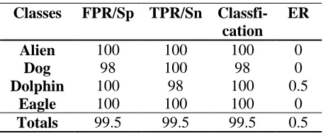
Table II: Classification Parameters
Classes
FPR/Sp TPR/Sn
Classfi-cation
ER
Alien
100
100
100
0
Dog
98
100
98
0
Dolphin
100
98
100
0.5
Eagle
100
100
100
0
Totals
99.5
99.5
99.5
0.5
It is observed that one sample of Dolphin class is misclassified as Dog class, which is shown in figure 6(a). The error rate is calculated and it is observed that the average error rate is reduced
if the experiments are performed more number of times. This can clearly be seen in figure 6(b). The x-axis gives the frequency of experiments conducted and y-axis gives the average error rate. It is observed in the figure 6(b) that as the frequency of experiments increased the average error rate is decreased.
The performance of the classification is given in Table II.
4.
C
ONCLUSIONOur approach to objects recognition is based on the shape representation technique, which identify various features from the shape using the mathematical morphology. The features are extracted by tuning the object and background, present in training images. This helps in minimizing the time and space complexity in both the training and test phases. The classification is performed on the various shape images by using quadratic classifier. The result of classification is shown by means of confusion matrix and it is observed that overall classification rate of all the objects is above 99%.
Fig. 6(a): QDC Classfier
Fig. 6(b). Error Graph [image:4.612.61.552.322.671.2]
[image:4.612.303.535.480.669.2]
5.
R
EFERENCES[1] J. Eggermont, A. E. Eiben, and J. I. van Hemert, “A comparison of genetic programming variants for data classification,” in Proc. 3rdSymp. IDA, 1999, Lecture Notes in Computer Science, vol. 1642, pp. 281–290.
[2] D. Howard, S. C. Roberts, and C. Ryan, “The Boru data crawler for object detection tasks in machine vision,” in Proc. Appl. Evol. Comput., EvoWorkshops: EvoCOP, EvoIASP, EvoSTim, S. Cagnoni, J. Gottlieb, E. Hart,M.Middendorf, and G. Raidl, Eds., Apr. 3/4, 2002, Lecture Notes in Computer Science, vol. 2279, pp. 220–230.
[3] H. F. Gray, R. J. Maxwell, I. Martinez-Perez, C. Arus, and S. Cerdan, “Genetic programming for classification of brain tumours from nuclear magnetic resonance biopsy spectra,” in Proc. 1st Annu. Conf. Genetic Program., J. R. Koza, D. E. Goldberg, D. B. Fogel, and R. L. Riolo, Eds., Jul. 28–31, 1996, p. 424.
[4] D. Valentin, H. Abdi, and A. J. O’Toole, “Categorization and identification of human face images by neural networks: A review of linear autoassociator and principal component approaches,” J. Biol. Syst., vol. 2, no. 3, pp. 413–429, 1994. [5] R. Poli, “Genetic programming for image analysis,” in Proc.
1st Annu.Conf. Genetic Program., J. R. Kosa, D. E. Goldberg, D. B. Fogel, and R. L. Riolo, Eds., Jul. 28–31, 1996, pp. 363– 368.
[6] J. Serra, Image Analysis and Mathematical Morphology. London, U.K.: Academic, 1982.
[7] R. M. Haralick, S. R. Sternberg, and X. Zhuang, “Image analysis using mathematical morphology,” IEEE Trans. Pattern Anal. Mach. Intell., vol. 9, no. 4, pp. 532–550, Apr. 1987.
[8] P. A. Maragos and R. W. Schafer, “Morphological skeleton representation and coding of binary images,” IEEE Trans. Acoust. Speech Signal Process., vol. ASSP-34, no. 5, pp. 1228–1244, Oct. 1986.
[9] I. Pitas and A. N. Venetsanopoulos, “Morphological shape decomposition,” IEEE Trans. Pattern Anal. Mach. Intell., vol. 12, no. 1, pp. 38–45, Jan. 1990.
[10] J. M. Reinhardt and W. E. Higgins, “Comparison between the morphological skeleton and morphological shape decomposition,” IEEE Trans. Pattern Anal. Mach. Intell., vol. 18, no. 9, pp. 951–957, Sep. 1996.
[11] P. Maragos, “Morphology-based symbolic image modeling, multi-scale nonlinear smoothing, and pattern spectrum,” in Proc. IEEE Comput. Soc. Conf. Computer Vision Pattern Recognition, 1988, pp. 766–773.
[12] I. Pitas and A. N. Venetsanopoulos, “Morphological shape representation,” Pattern Recognit., vol. 25, no. 6, pp. 555–565, 1992.
[13] J. M. Reinhardt and W. E. Higgins, “Efficient morphological shape representation,” IEEE Trans. Image Process., vol. 5, no. 6, pp. 89–101, Jun. 1996.
[14] J. Xu, “Morphological decomposition of 2-D binary shapes into conditionally maximal convex polygons,” Pattern Recognition., vol. 29, no. 7, pp. 1075–1104, 1996.
[15] J. Xu, “Morphological representation of 2-D binary shapes using rectangular components,” Pattern Recognition, vol. 34, no. 2, pp. 277–286, 2001.
[16] J. Xu, “Morphological decomposition of 2-D binary shapes into convex polygons: A heuristic algorithm,” IEEE Trans. Image Process., vol. 10, no. 1, pp. 61–71, Jan. 2001.
[17] J. Xu, “Efficient morphological shape representation with overlapping disk components,” IEEE Trans. Image Process., vol. 10, no. 9, pp. 1346–1356, Sep. 2001.
[18] J. Xu, “A generalized discrete morphological skeleton transform with multiple structuring elements for the extraction of structural shape components,” IEEE Trans. Image Process., vol. 12, no. 12, pp. 1677–1686, Dec. 2003.
[19] J. Xu, “Efficient morphological shape representation by varying overlapping levels among representative disks,” Pattern Recognition., vol. 36, no. 2, pp. 429–437, 2003. [20] Held and K. Abe, “On the decomposition of binary shapes into
meaningful parts,” Pattern Recognition., vol. 27, no. 5, pp. 637–647, 1994.
[21] Ronse and B. Macq, “Morphological shape and region description,” Signal Process., vol. 25, pp. 91–106, 1991. [22] J. Goutsias and D. Schonfeld, “Morphological representation
of discrete and binary images,” IEEE Trans. Signal Process., vol. 39, no. 6, pp. 1369–1379, Jun. 1991.
[23] J. Xu, “Morphological decomposition of 2-D binary shapes into modestly Overlapped Octagonal and Disk Componenet,” IEEE Trans. On Image Processing, vol. 16, no. 2, pp. 337– 348, Feb. 2007.
[24] Cheng-Lin Liu, Sako H, and Fujisawa H, "Discriminative Learning Quadratic Discriminant Function for Handwriting Recognition", IEEE Transaction on Neural networks, Vol.15, No.2, pp.430-444, 2004.