Noise Estimation by Utilizing Mean Deviation of Smooth Region in Noisy Image
Suhaila Sari, Hazli Roslan
Faculty of Electrical and Electronic Engineering Universiti Tun Hussein Onn Malaysia
Johor, Malaysia {suhailas,hazli}@uthm.edu.my
Tetsuya Shimamura
Graduate School of Science and Engineering Saitama University
Saitama, Japan
shima@@sie.ics.saitama-u.ac.jp
Abstract—In many practical cases of image processing, only a noisy image is available. Many image denoising methods usually require the exact value of the noise distribution as an essential filter parameter. However, to estimate the noise solely from the information of the noisy image is a difficult task. A simple but accurate noise estimator would significantly benefit many image denoising methods. In this paper, we present a method to estimate additive noise by utilizing the mean deviation of a smooth region selected from a noisy image. The noise distribution is estimated by computing the average mean deviation of all non-overlapping blocks in the smooth region. Simulation results demonstrate that our method achieves ac-curate noise estimation regardless of the image characteristics over a range of noise levels. The restoration performance of a denoising technique based on our noise estimation method resembles that achieved in the ideal condition.
Keywords-noise estimation; mean deviation; smooth region.
I. INTRODUCTION
In many practical cases of image processing, only a noisy image is available. This circumstance is known as the blind condition. Many denoising methods usually require the exact value of the noise distribution as an essential filter parameter. Thus, the properties of the original image or noise, such as the power spectrum or variance, must first be estimated solely from the information of the noisy image to apply denoising. This difficult task has been studied for many years. Some of the noise estimation methods in different domains are found in the following literatures: methods in the spatial domain [1][2] and those in the transform domain [3]-[5]. Among them, the two most common approaches are those suggested by Lee [1] and Donoho [4].
In [1], the local variances are estimated from the neigh-bourhood around each pixel. The average of these estimates is subsequently used as the noise variance of the noisy image. Although this approach is simple, the accuracy of variance estimation may be influenced by the local variance in non-smooth regions which consist of fine detail and edges. On the other hand, the transform-based variance estimator in [4] computes the noise standard deviation, σest, as the median absolute deviation (M AD) of the wavelet coeffi-cients in the highest frequency subband. The noise standard deviation is calculated as σest=M AD/0.6745. The noisy image must be transformed into the wavelet domain by
downsampling the image for several decomposition levels. The estimator in [4] has proven to be a robust estimator in the wavelet domain. However, its computational complexity is increased because it is employed in the transform domain. In addition to the above-mentioned methods, some inter-esting noise estimation methods performed in the spatial domain have also been introduced. The block-based noise estimation method, as proposed by Lee and Hoppel [6], calculates the standard deviation of the blocks in the noisy image. The smallest standard deviation is assumed to be equal to the actual additive white Gaussian noise (AWGN). Although this algorithm is simple, it tends to overestimate or underestimate the noise distribution.
Filtering-based noise estimation methods, such as [7] and [8], suggest filtering of the noisy image to smooth the image before estimating the noise. Olsen’s method [7] has difficulty of estimating the noise in images with fine details and edges, because these features may be smoothed out by the filtering process. This causes inaccurate noise estimation because the image structure is included in the noise estimation. On the other hand, the method proposed in [8] first filters the image by a vertical and horizontal difference operator and utilizes the difference signal to produce a local variance histogram, which is then used to estimate the variance of the noise. This method depends heavily on fixing many parameters. Both of the noise estimation methods in [7] and [8] require a high computational cost. Therefore, the development of a simple but accurate method that estimates the noise directly from the noisy image will significantly benefit the implementation of denoising methods in the spatial domain.
In most noise estimation methods in the spatial domain, the variance or standard deviation is used to estimate the actual added noise distribution. However, here we investigate an alternative measure of dispersion to provide accurate noise estimation. To our knowledge, noise estimation meth-ods (performed in the spatial domain) that exploit the mean deviation of the smooth region of a noisy image have not yet been proposed. In this paper, we propose a noise estimation method called the smooth region mean deviation-based estimator (SR-MDE).
The paper is organized as follows. The SR-MDE algo-rithm is described in Section 2. The performance comparison
for the SR-MDE is discussed in Section 3. Finally, conclud-ing remarks are drawn in Section 4.
II. PROPOSED ALGORITHM
Assume that an original imagey(i, j)is corrupted by an additive zero-mean white Gaussian noisen(i, j). The mean (‘average’,µ) and variance (standard deviation squared,σ2) are the defining parameters of the AWGN. The AWGN has a random value within the distribution and does not depend on the original image intensity [9].
In image processing, one approach to obtain noise infor-mation is to estimate the noise properties from a specified smooth region [9], [10]. We estimate the noise directly from the spatial domain because it is visually easier to distinguish a smooth region from a noisy image. If a region of nearly constant background level is selected and the noise appears to be Gaussian, the variability in the selected smooth region is due primarily to the distribution of noise. Moreover, utilization of the smooth region alone can overcome the influence of non-smooth regions to the noise estimation.
We propose to use the mean deviation rather than the vari-ance or standard deviation to estimate the noise distribution. The advantage of this approach is that the mean deviation is actually more efficient than the standard deviation in practical situations [11]. The standard deviation emphasises a larger deviation; squaring the values makes each unit of distance from the mean exponentially (rather than additively) greater [11]. The larger deviation will cause overestimation or underestimation of the noise. Therefore, we assume that use of the mean deviation may contribute to more accurate noise estimation.
The mean deviation, M D, is the mean of the absolute difference between a set of pixel values, f(i, j), and their mean,µf, and is given by
M D= 1 ab a X i=1 b X j=1
|f(i, j)−µf|, (1)
where
µf =
1 ab a X i=1 b X j=1
f(i, j). (2)
TheM D is also called the mean absolute deviation or mean difference [12]. In contrast, the standard deviation, σ, is obtained by σ= v u u t 1 ab a X i=1 b X j=1
(f(i, j)−µf)2. (3)
For the Gaussian distribution, the ratio of the M D to σ is p
(2/π)[13]. Hence,
σ= 1.253×M D. (4)
In medical images such as those of magnetic resonance (MR), a smooth region can be identified from the back-ground [10]. However, in standard images, the backback-ground usually does not exist. In this case, one approach is to select a region in the noisy image with a background with as few features as possible. However, selecting a smooth region from a standard image is difficult. For example, in the automated block-based noise estimation approach [6], calculating the smallest standard deviation from a set of blocks does not necessarily guarantee that the selected block is obtained from a smooth region. In some noisy image cases, a non-smooth region can generate the smallest variance owing to the mixture of additive noise and image details, which have similar intensities.
Therefore, in the SR-MDE, we directly specify the region of interest (ROI) of multiple smooth-region blocks from the noisy image x(i, j) (see Fig. 1). The selected blocks are represented byROI1,ROI2,...,ROIm, wheremis the ROI number. The size of each ROI block is fixed to 16×16
pixels. The selection of this block size ensures that the sample is large enough to calculate the noise effectively. From all ROIm, the ROI block that provides the smallest mean deviation,r(k, l), is utilized for noise estimation.
The resulting r(k, l) is divided into non-overlapping blocks,r(s,t)(k, l),2×2pixels in size, where(s, t)is defined as s = 1,2, ...,8 and t = 1,2, ...,8. We tested different window sizes and found that for the SR-MDE, the best noise estimation results are achieved with the minimal possible window size, (i.e. a block size of2×2 pixels). The mean deviation ofr(s,t)(k, l),M Dr(s,t), is obtained by
M Dr(s,t)=
1 4 2 X k=1 2 X l=1
r(s,t)(k, l)−µr(s,t)
, (5)
where the mean of r(s,t)(k, l),µr(s,t), is given by
µr(s,t)=
1 4 2 X k=1 2 X l=1
r(s,t)(k, l). (6)
The noise distribution of the noisy image,M Dr, is approx-imated by computing the mean of the entireM Dr(s,t), as
M Dr=mean(M Dr(s,t)). (7)
The estimated standard deviation of the additive noise can be obtained by using
σr= 1.253×M Dr. (8)
III. RESULTS AND DISCUSSION
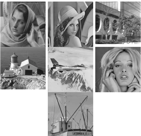
We performed experiments to investigate the accuracy of the SR-MDE. We conducted experiments on standard grayscale images (256×256) with different image charac-teristics from the SIDBA database (see Fig. 2).
Figure 1. Example of selected smooth regions from Lena image corrupted by noise ofσ= 10.
Figure 2. Test images with different characteristics. From left to right, top to bottom: Barbara, Lena, Building, Lighthouse, Airplane, Woman, and Boat.
several approaches to estimate the noise standard deviation of the noisy image. The noise was estimated by using the following statistics.
(a) The standard deviation of the selected smooth region
r(k, l),σr, computed by (8).
(b) The standard deviation of the selected smooth region
r(k, l). The noise standard deviation was calculated by (3), and represented as σ ref.
(c) The mean deviation from the entire image. The noisy
image was divided into non-overlapping blocks, 16×16
pixels in size. The M D for each block was calculated by a process similar to that in Sect. II. The mean of the entire
M D was calculated and multiplied by 1.253. The product was denoted as M D local.
(d) A simple noise estimation method proposed by Lee [1]. The local noise standard deviation given by (3) was computed from a window 3×3 in size around each pixel. The mean of all local noise standard deviations over the entire image was utilized as the estimated noise standard deviation, σ local.
(a) Noise estimation (σ= 5)
(b) Noise estimation (σ= 10)
[image:3.612.322.553.217.698.2](c) Noise estimation (σ= 15)
[image:3.612.62.289.338.557.2]Table I
PERFORMANCE COMPARISON OFMSSIMFORBM3D
Test images BM3D BM3D (σr)/ BM3D (M D local)/ BM3D (σ ref)/ BM3D (σ local)/
(ideal) (σr) ideal (M D local) ideal (σ ref) ideal (σ local) ideal
Noise standard deviation,σ= 5
Barbara 0.97 0.97 1.00 0.95 0.97 0.95 0.97 0.97 0.99
Lenna 0.97 0.97 1.00 0.96 0.99 0.90 0.93 0.95 0.98
Building 0.97 0.97 1.00 0.95 0.98 0.95 0.98 0.94 0.96
Lighthouse 0.96 0.96 1.00 0.90 0.94 0.92 0.95 0.95 0.99
Airplane 0.96 0.96 1.00 0.94 0.98 0.89 0.92 0.89 0.92
Woman 0.96 0.96 1.00 0.94 0.98 0.91 0.94 0.96 1.00
Boat 0.97 0.97 1.00 0.95 0.99 0.89 0.91 0.96 0.99
Noise standard deviation,σ= 10
Barbara 0.95 0.94 0.99 0.93 0.98 0.82 0.87 0.95 1.00
Lenna 0.94 0.94 1.00 0.94 1.00 0.75 0.80 0.94 1.00
Building 0.94 0.94 1.00 0.93 0.99 0.85 0.90 0.82 0.87
Lighthouse 0.92 0.92 1.00 0.88 0.96 0.78 0.85 0.77 0.84
Airplane 0.93 0.93 1.00 0.92 0.99 0.72 0.77 0.88 0.94
Woman 0.93 0.92 1.00 0.92 0.99 0.73 0.79 0.72 0.78
Boat 0.94 0.94 1.00 0.93 0.99 0.72 0.76 0.91 0.97
Noise standard deviation,σ= 15
Barbara 0.93 0.91 0.99 0.92 0.99 0.70 0.75 0.91 0.99
Lenna 0.92 0.91 0.99 0.92 1.00 0.59 0.65 0.92 1.00
Building 0.90 0.89 0.99 0.90 1.00 0.72 0.80 0.68 0.76
Lighthouse 0.88 0.88 1.00 0.85 0.97 0.68 0.77 0.63 0.72
Airplane 0.91 0.90 1.00 0.90 1.00 0.58 0.64 0.88 0.97
Woman 0.90 0.89 0.99 0.90 1.00 0.61 0.68 0.86 0.95
Boat 0.91 0.90 0.99 0.91 1.00 0.57 0.62 0.70 0.77
Fig. 3 shows the noise estimation results. Note that the SR-MDE provided the most accurate noise estimation, especially at low to moderate noise levels (σ = 5 to 10). The SR-MDE provides robust estimation regardless of the image characteristics because it considers only the selected smooth region. In all cases, the estimated noiseσ ref has a relatively greater distance from the actual noise standard deviation than doesσr. This is due to the greater deviation produced by the squaring in (3). In contrast, the noise estimates acquired from the entire noisy image (M D local
and σ local) were significantly influenced by the image characteristics. This effect can easily be explained by the existence of fine details and edges in the non-smooth regions of the original image. These features produce a large devia-tion among the pixel values in the non-smooth regions. The averaging process in theM D local and σ local estimates include the noise estimated from the non-smooth regions in the entire image. This causes inaccuracy in the noise estimation.
To investigate the performance of the SR-MDE in a practical case, we performed denoising by using the con-ventional denoising technique: the block-matching 3D filter (BM3D) [14], employing the estimated noise standard de-viation ofσr,M D local,σ ref andσ local, respectively. We utilized the same corrupted images as those used in the
previous noise estimation process. In the ‘BM3D (ideal)’ case, the actual noise standard deviation σ was provided for each denoising process. For the ‘BM3D (σr)’, ‘BM3D (M D local)’, ‘BM3D (σ ref)’ and ‘BM3D (σ local)’ cases, theσr,M D local,σ refandσ localwere obtained from each noisy image, respectively, and provided to each denoising process.
Table 1 shows a performance comparison of the BM3D denoising method in terms of the objective image quality as assessed by the mean measure of structural similarity (MSSIM) [15]. The MSSIM mimics human perception and models image distortion as a combination of correlation loss, luminance distortion, and contrast distortion. The maximum value for the MSSIM is 1. Note that the BM3D that employs the SR-MDE provided denoising performance comparable to that of the ideal case.
IV. CONCLUSION
by developing an accurate procedure to automatically select the smooth region.
ACKNOWLEDGMENT
The authors would like to thank Universiti Tun Hussein Onn Malaysia and Malaysia Government for sponsoring for this paper. We also would to thanks Saitama University for the support and cooperation upon completion of this paper.
REFERENCES
[1] J. S. Lee, “Digital image enhancement and noise filtering by use of local statistics,”IEEE Trans. Pattern Analysis and Ma-chine Intelligent, vol. PAMI-2, no. 2, pp. 165–168, Mar. 1980.
[2] Z. Lu, G. Hu, X. Wang, and L. Yang, “An improved adaptive Wiener filtering algorithm,” inProc. Int. Conf. Signal Process., IEEE 2006, pp. 60–65.
[3] J. S. Lim, and N. A. Malik, “A new algorithm for two-dimensional maximum entropy power spectrum estimation,” IEEE Trans. Acoustic Speech, and Signal Process., vol. 29, no. 3, pp. 401–413, June 1981.
[4] D. L. Donoho, “De-noising by soft-thresholding,” IEEE
Trans. Information Theory, vol. 41, no. 3, pp. 613–627, May 1995.
[5] S. Suhaila, and T. Shimamura, “Power spectrum estimation method for image denoising by frequency domain Wiener fil-ter,” inProc. Int. Conf. Computer and Automation Engineering IEEE, 2010, pp. 608–612.
[6] J. S. Lee, and K. Hoppel, “Noise modeling and estimation of remotelysensed images,” inProc. Int. Geoscience and Remote Sensing, 1989, vol. II, pp. 1005–1008.
[7] S. I. Olsen, “Estimation of noise in images: an evaluation,” GraphModels and Image Process.,vol. 55, pp. 319–323, July 1993.
[8] K. Rank, M. Lendl, and R. Unbehauen, “Estimation of image noise variance,”IEE Proc. Vision, Image and Signal Process., vol. 146, no. 2, pp. 80–84, Aug. 1999.
[9] R. C. Gonzalez, R. E. Woods, and S. L. Eddins,Digital Image Processing using MATLAB, Prentice Hall, New Jersey, 2004.
[10] L. He, and I. R. Greenshields, “A nonlocal maximum like-lihood estimation method for rician noise reduction in MR images,”IEEE Trans. Medical Imaging,vol. 28, no. 2, pp. 165– 172, Feb. 2009.
[11] S. Gorard, “Revisiting a 90-year-old debate: the advantages of the mean deviation,”British Journal of Educational Studies, vol. 53, no. 4, pp. 417–430, Dec. 2005.
[12] J. F. Kenney, and E. S. Keeping,Mathematics of Statistics, Princeton, New Jersey, 1962.
[13] L. Sachs, Applied Statistics: A Handbook of Techniques, Springer-Verlag, New York, 1984.
[14] K. Dabov, A. Foi, V. Katkovnik, and K. Egiazarian, “Image denoising by sparse 3D transform-domain collaborative filter-ing,”IEEE Trans. Image Process.,vol. 16, no. 8, pp. 2080– 2095, Aug. 2007.