www.hydrol-earth-syst-sci.net/20/669/2016/ doi:10.5194/hess-20-669-2016
© Author(s) 2016. CC Attribution 3.0 License.
Comparing statistical and process-based flow duration curve models
in ungauged basins and changing rain regimes
M. F. Müller and S. E. Thompson
Department of Civil and Environmental Engineering, Davis Hall, University of California, Berkeley CA, USA
Correspondence to: M. F. Müller ([email protected])
Received: 22 August 2015 – Published in Hydrol. Earth Syst. Sci. Discuss.: 25 September 2015 Revised: 25 January 2016 – Accepted: 27 January 2016 – Published: 11 February 2016
Abstract. The prediction of flow duration curves (FDCs) in ungauged basins remains an important task for hydrologists given the practical relevance of FDCs for water manage-ment and infrastructure design. Predicting FDCs in ungauged basins typically requires spatial interpolation of statistical or model parameters. This task is complicated if climate be-comes non-stationary, as the prediction challenge now also requires extrapolation through time. In this context, process-based models for FDCs that mechanistically link the stream-flow distribution to climate and landscape factors may have an advantage over purely statistical methods to predict FDCs. This study compares a stochastic (process-based) and sta-tistical method for FDC prediction in both stationary and non-stationary contexts, using Nepal as a case study. Under contemporary conditions, both models perform well in pre-dicting FDCs, with Nash–Sutcliffe coefficients above 0.80 in 75 % of the tested catchments. The main drivers of uncer-tainty differ between the models: parameter interpolation was the main source of error for the statistical model, while vio-lations of the assumptions of the process-based model rep-resented the main source of its error. The process-based ap-proach performed better than the statistical apap-proach in nu-merical simulations with non-stationary climate drivers. The predictions of the statistical method under non-stationary rainfall conditions were poor if (i) local runoff coefficients were not accurately determined from the gauge network, or (ii) streamflow variability was strongly affected by changes in rainfall. A Monte Carlo analysis shows that the streamflow regimes in catchments characterized by frequent wet-season runoff and a rapid, strongly non-linear hydrologic response are particularly sensitive to changes in rainfall statistics. In these cases, process-based prediction approaches are favored over statistical models.
1 Introduction
The flow duration curve (FDC) provides a compact summary of the variability of daily streamflow by indicating what pro-portion of the flow regime exceeds a given flow rate. FDCs have considerable practical relevance, particularly in sup-porting decisions that are affected by the availability and reliability of surface water. Common applications of FDCs include the design and management of hydropower infras-tructure (e.g., Basso and Botter, 2012; Müller, 2015), the de-termination of environmental flow standards for ecosystem protection (e.g., Lazzaro et al., 2013), the allocation of water resources for consumptive uses (e.g., Alaouze, 1989), or the prediction of streamflow time series in ungauged or poorly gauged catchments (e.g., Hughes and Smakhtin, 1996; West-erberg et al., 2014).
Despite their utility, empirical FDCs are unavailable for many basins, primarily because they require extensive on-site observations of daily streamflow (Vogel and Fennessey, 1994). Globally, the majority of catchments remain un-gauged (or the gauge data that exist are subject to significant quality assurance and data availability constraints). Further-more, the global number of stream gauges continues to de-cline because of ongoing budgetary constraints faced by wa-ter monitoring agencies (Stokstad, 1999; United States Ge-ological Survey, 2015). Therefore FDCs must typically be estimated in data-scarce areas. The most widely used tech-niques for FDC estimation are simple, graphical methods. Such empirical methods are easy to implement but often rely on overly simplistic assumptions that lead to substantial prediction errors. For instance, in Nepal, the regionalization method prescribed in official design manuals (e.g., Chitrakar, 2004; Alternative Energy Promotion Center, 2014) relies on
to scale standardized regional indices for monthly flows. The procedure neglects the inter-annual variability of low flows, which leads to important biases in the predicted flow distri-butions (see Sect. S1 of the Supplement). Even in gauged catchments, FDCs constructed from historical observations may not represent current flow conditions well, because flow regimes are impacted by climate change and anthropogenic alterations of the catchments (e.g., Botter et al., 2013; Mu et al., 2007). Predicting streamflow in ungauged basins, par-ticularly in the context of environmental change, remains both a fundamental necessity for water managers and a ma-jor research challenge (Blöschl et al., 2013; Montanari et al., 2013).
Recent efforts to predict FDCs in ungauged catchments fo-cus on statistical approaches that predict the flow distribution based on the catchment’s similarity to nearby, gauged water-sheds (Castellarin et al., 2013). Index flow approaches, which regionalize specific index flows (typically the mean flow), and use those indices to rescale empirical FDCs from simi-lar catchments, are particusimi-larly popusimi-lar (e.g., Chalise et al., 2003; Castellarin et al., 2004b; Sauquet and Catalogne, 2011; Arora et al., 2005). While differing in methodological de-tails, all index flow approaches assume that FDCs do not vary within homogeneous regions, except by a scaling factor. Be-cause they do not assume any specific runoff-generating pro-cess, statistical methods are versatile. They have been suc-cessfully applied globally to predict FDCs in a variety of climates and catchment types (Blöschl et al., 2013). How-ever, methods are also insensitive to the diversity of con-trols on the shape of the FDC exerted by climate processes and catchment characteristics. This may affect their reliabil-ity under non-stationary conditions (Milly et al., 2008). Fi-nally, the calibration of statistical methods relies on exten-sive streamflow observations from a large number of rep-resentative and well-characterized catchments (e.g., Cheng et al., 2012; Coopersmith et al., 2012). Their performance is therefore sensitive to the spatial density of available gauges (Blöschl et al., 2013), and their reliability in regions where streamflow data are truly scarce is uncertain.
Stochastic, process-based models that mechanistically link the drivers, state, and response of the system are a promis-ing avenue to address these issues. In these models, basic assumptions about the stochastic structure of rainfall and the (deterministic) response of catchments allow the ana-lytic derivation of streamflow probability density functions (PDFs). (Note that because the FDC can be obtained directly by transforming the PDF, a predictive technique that yields the streamflow PDF will also allow the FDC to be estimated.) Botter et al. (2007b) show that runoff follows a gamma dis-tribution if catchments behave as a linear reservoir, forced by stochastic rainfall that follows a marked Poisson process. The resulting gamma distribution depends on two parameters that are determined by the recession characteristics of the catch-ment, and by the frequency and intensity of effective rain. This process-based approach to the streamflow PDF has been
extended to include the fast flow component of streamflow (Muneepeerakul et al., 2010), non-linearities in subsurface storage–runoff relationships (Botter et al., 2009), the effects of short-term snowmelt (Schaefli et al., 2013), and the car-ryover of subsurface storage between seasons in seasonally dry climates (Müller et al., 2014). Although the stochastic framework allows the effects of changes in climate or land-scape to be independently modeled, it relies on strong sim-plifying assumptions about the spatial homogeneity of catch-ments. These assumptions make the existing process mod-els less versatile than statistical methods. Nonetheless, the approach has low calibration requirements because it relies on a small number of parameters, which can be determined using rainfall, climate, and geomorphological characteristics of the catchments (Doulatyari et al., 2015). This informa-tion is increasingly available in ungauged basins, thanks to remote-sensing technologies, even when ground-based mea-surements are sparse.
Process-based models successfully reproduce streamflow PDFs in numerous gauged catchments worldwide (Botter et al., 2007a; Ceola et al., 2010), including Nepal (Müller et al., 2014). Yet their predictive performance in ungauged basins remains largely unassessed, particularly in regions where the local gauge density is globally representative (as opposed to densely monitored catchments in developed countries such as, e.g., France and Austria in Castellarin et al., 2013). For lower gauge densities, it is unclear whether the advantages of the process-based approaches, which are derived from an explicit representation of flow-generating processes, are outweighted by the limitations imposed by the restrictive assumptions underlying these methods – and whether this trade-off is altered by non-stationarity in climate drivers.
Using Nepal as a test case, this study compares the process-based and statistical approaches on the basis of (i) their ability to predict FDCs in ungauged basins, (ii) their sensitivity to data scarcity, represented both by the spatial density of the stream gauge network and by the tempo-ral extent (length) of the available streamflow records, and (iii) their ability to accommodate changes in the rainfall regime.
200km
Chepe Kohla Catchment
Stream Gauges (N=25) Catchments
Rain Gauges (N=178) Stream Gauges per 10000 km2
No. of countries
0.01 1 100
0
25
50 Nepal:1.6
(a) (b)
Behri Catchment
20km
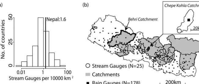
Figure 1. (a) Global histogram of the approximate spatial density of streamflow gauges by nation, represented by the sample of 8540 gauges indexed by the Global Runoff Data Center for 146 countries (Global Runoff Data Center, 2014). With a density of 1.6 gauges per 10 000 km2, Nepal falls close to the mode of the global distribution. (b) Location of the rain gauges, streamflow gauges, and corresponding Nepalese catchments used in the analysis.
heterogeneous, and highly seasonal. There is also signifi-cant carryover of groundwater storage between the wet and dry seasons, so that dry-season discharge reflects the fea-tures of the antecedent wet season. These characteristics vio-late many of the assumptions that underlie the process-based method. The analysis in Nepal is therefore likely to provide a conservative estimate of the potential performance of the process-based method in ungauged basins. Finally, develop-ing reliable methods for FDC prediction in Nepal represents an opportunity for “use-inspired science” (Thompson et al., 2013b). Nepal has an enormous untapped hydropower po-tential and is in dire need of electrical power, particularly in rural areas. A reliable method to estimate FDCs in ungauged catchments would be a valuable tool to support the devel-opment of micro-hydropower, a sustainable technology for rural electrification (Müller, 2015).
Section 2 describes the two models and the procedures used to estimate their parameters from streamflow and rain-fall observations. Section 3 presents the results of the com-parative analysis in Nepal. Section 4 examines the key sources of errors for both models and discusses implications for both “Prediction in ungauged catchments” (PUB) and “Predictions under change” (PUC) beyond Nepal.
2 Methods
2.1 Compared approaches 2.1.1 Process-based model
The process-based approach models daily streamflow as a random variable. Subject to strong simplifying assumptions about rainfall stochasticity and runoff generation, the stream-flow PDF can be analytically derived. During the wet season, daily rainfall is represented as a stationary marked Poisson process with exponentially distributed depths. Assuming
[image:3.612.138.464.67.205.2]The model was successfully validated in a variety of re-gions with seasonally dry climates worldwide, including Nepal, where observed FDCs were predicted in 24 gauged catchments with a median Nash–Sutcliffe coefficient of 0.90 on log-transformed flow quantiles (Müller et al., 2014). The approach successfully reproduced both the rain-driven dis-tribution of flows during the wet season and the release of stored monsoon water during the dry-season recession. In this study, we assess the operational performance of the process-based approach as a tool to predict streamflow in
un-gauged catchments. Therefore, we do not further attempt to
attribute model errors to parameters versus the model struc-ture in the results presented in Sect. 3, since in practice these errors are confounded in any real application. The relative significance of these two error sources is nonetheless dis-cussed in Sect. 4.1.1.
In ungauged catchments, the process-based model is im-plemented as follows. Three of the seven parameters of the model (Td,λP,αP) are rainfall characteristics that can be es-timated in ungauged basins using meteorological observa-tions. Recession parameters (kandb) describe aquifer prop-erties that are challenging to observe at the catchment scale. They can be estimated using observed streamflow time series in nearby gauged basins and subsequently interpolated from nearby gauges using the geostatistical approach described in Müller and Thompson (2015), which accounts for the topol-ogy of the stream network. The last two parameters (ET) and (SSC) describe catchment-scale soil moisture dynamics that are arduous to determine empirically. Previous applica-tions of the model relied on reasonable values of ET and SSC, based on land use, soil, and climate characteristics of the catchment (e.g., Botter et al., 2007a; Ceola et al., 2010). Alternatively, runoff coefficients can be used to directly re-late rainfall statistics to streamflow increments (Doulatyari et al., 2015). Runoff coefficients describe the ratio of mean discharge to mean precipitation, and can be predicted in un-gauged basins using water balance models and meteorologi-cal observations. This approach circumvents the need to esti-mate ET and SSC, but the accuracy of predicted runoff coef-ficients in ungauged catchments is critically dependent on the type of water balance model used and on the availability of appropriate calibration data (Doulatyari et al., 2015). Instead, this study follows the former procedure and uses reasonable estimates of ET and SSC for Nepal.
2.1.2 Statistical model
The statistical approach is entirely driven by observation data and does not assume any specific runoff generation process. Instead, it identifies and exploits statistical correlations that may occur between streamflow observed at existing gauges and the geology, topography, and climate of the correspond-ing catchments. The index flow model used in this study was developed by Chalise et al. (2003) to regionalize FDCs in Nepal to assess the potential for small hydropower
develop-ment. The model is based on local flow indices for mean (Qm=E[Q]) and low (q95=Q95/Qm, where Q95 is the 95th streamflow percentile) flows, and uses a non-parametric approach to represent the shape of the FDC. Empirical FDCs from available gauges are normalized byQmand pooled into equally sized groups based on theq95 index of the gauge. A standardized curve is determined for each group by tak-ing the average of the normalized flows correspondtak-ing to each duration, in order to represent the average catchment response in the group. The chosen statistical approach is con-siderably less complex than many alternative state-of-the-art methods using multiple (often non-linear) equations to relate multiple flow quantiles to a variety of observed covariates (see Castellarin et al., 2013, for a review). However, Chalise et al. (2003) is, to our knowledge, the most recent statisti-cal method specifistatisti-cally developed and validated in the study region. The approach is parsimonious and adapted to situ-ations, where in situ observations of catchment characteris-tics are scarce. The method is therefore representative of the level of complexity of statistical approaches likely to be im-plemented in developing countries for practical hydrological engineering purposes.
Predictions in ungauged catchments are obtained by first using linear regressions to predict Qm and q95. Although the original method calls for a stepwise multiple regression approach to determine regression covariates inductively, we used the regression models obtained in Chalise et al. (2003): Qm is regressed against annual rainfall (Ry) and gauge el-evation (zmin) as a proxy for evapotranspiration, andq95 is regressed against the ratios of catchment area occupied by each of the considered geological units. The two regressions loosely represent the long-term water balance and short-term response of the catchment. The predicted low-flow index is then used to determine the standardized FDC shape, which is finally multiplied by the predicted mean flow to obtain the FDC. An important assumption, inherent to the linear regres-sion models, is that the dependent variable (hereQmandq95) is not spatially correlated when controlling for the considered covariates. This assumption is reasonable in Nepal, where the typical distance between stream gauges is much larger than the correlation scale of runoff (Müller and Thompson, 2015). In more densely gauged areas (or if runoff is correlated over larger distances), streamflow observations at neighboring or flow-connected gauges are likely to be correlated. In these regions, accounting for the effect of distance and stream net-work topology when interpolating flow indices (e.g., using TopREML Müller and Thompson, 2015) will improve pre-dictions.
2.2 Study region and data
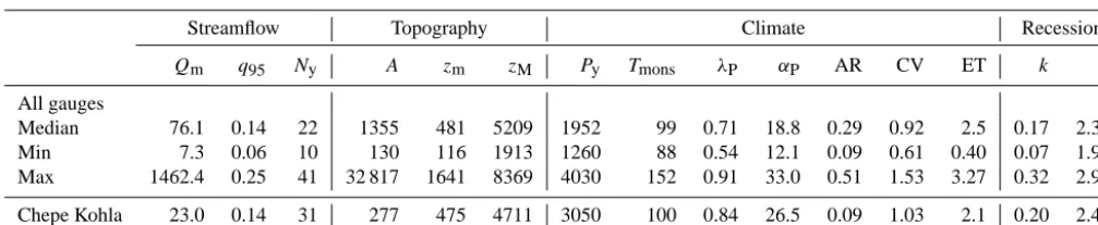
Table 1. Catchment characteristics. Median values and interquartile distances (IQD) are given for the whole sample of 25 gauges. The table also presents characteristics of the Chepe Kohla watershed considered in the analysis as a case study.
Streamflow Topography Climate Recession
Qm q95 Ny A zm zM Py Tmons λP αP AR CV ET k b
All gauges
Median 76.1 0.14 22 1355 481 5209 1952 99 0.71 18.8 0.29 0.92 2.5 0.17 2.38
Min 7.3 0.06 10 130 116 1913 1260 88 0.54 12.1 0.09 0.61 0.40 0.07 1.99
Max 1462.4 0.25 41 32 817 1641 8369 4030 152 0.91 33.0 0.51 1.53 3.27 0.32 2.99
Chepe Kohla 23.0 0.14 31 277 475 4711 3050 100 0.84 26.5 0.09 1.03 2.1 0.20 2.41
Qmis mean annual flow in m3s−1;q95is the 95th flow percentile normalized byQm;Nyindicates the number of observation years;Ais the catchment area in km2;zmandzM are, respectively, the minimum and maximum elevation of the basin’s meters;Pyis mean precipitation in mm yr−1;Tmonsis the estimated duration of the monsoon in days;λPis rainfall frequency during the monsoon (in d−1);α
Pis mean rainfall intensity in mm d−1; AR is the first-order autocorrelation coefficient of rainfall occurrence (AR=0if rainfall follows a Poissonian process), CV is the coefficient of variation of rainfall intensity on rainy days (CV=1if depths are exponentially distributed); ET (mm d−1) is the reference evapotranspiration during the rainy season (Lambert and Chitrakar, 1989);kis the linear recession constant estimated during the monsoon (in d−1) andbis the non-linear exponent of the seasonal recession. A soil moisture capacity of 16 mm is assumed throughout the country (Müller et al., 2014).
of daily streamflow records. They were checked for consis-tency, using double mass plots (Searcy and Hardison, 1960) and bias: we discarded non-glaciated catchments that had a precipitation deficit in their long-term water balance. Water-sheds were delineated using the ASTER GDEM v2 digital elevation model (NASA Land Processes Distributed Active Archive Center, LP DAAC). The study watersheds are lo-cated in central Nepal but cover a wide variety of catchment sizes, elevation ranges, precipitation characteristics, and ge-ological units (Table 1).
We focused on the Chepe Kohla catchment in central Nepal (Fig. 1b, insert) as a case study for analyses requiring resampling (Sect. 2.3.1) or simulation (Sect. 2.3.2) of stream-flow time series. The Chepe Kohla watershed has a long (by Nepalese standards) record of daily streamflow observations (31 years) and is representative of the full sample of gauges in terms of topography and recession behavior (Table 1). The catchment is also small (i.e., close to spatially homogenous), and local rainfall is well approximated by a marked Pois-son process (first-order autocorrelation coefficient of rain-fall occurrence (AR): 0.09; coefficient of variation of rainrain-fall depths (CV): 1.09), echoing the underlying assumptions of the process-based model.
Rainfall characteristics over the sampled catchments were obtained from 178 precipitation gauges (HKH-FRIEND, 2004; Department of Hydrology and Meteorology, 2011), also mapped in Fig. 1b. The average duration of the dry sea-son (Td) was estimated at each precipitation gauge by fitting a step function to the corresponding rainfall time series (Müller and Thompson, 2013), and wet-season precipitation records were used to compute the frequency and mean intensity of rainfall (λPandαP). Rainfall characteristics were then aggre-gated at the catchment level by assuming that the rain process aggregates linearly within the basins. For rainfall occurrence, we assumed that the duration between rain events caused by two consecutive storms can be estimated as the average of
the inter-arrival times measured at the rain gauges within the catchment. This allows us to compute catchment-level rain-fall frequency as
λP=
1 Ng
Ng X
i
1 λ(i)P
−1
,
whereλ(i)P designates rainfall frequency observed at gaugei andNgthe number of rain gauges within the catchment. Sim-ilarly, the catchment-level duration between rainy seasons is assumed to be the average of the durations observed within the catchment:
Td= 1 Ng
Ng X
i
Td(i).
Finally, the precipitation depth received on any given day by a catchment is assumed to be the average of the precipi-tation depths observed by individual rain gauges. It follows that the aggregated mean rainfall intensity can be expressed as
αP=λ−P1 1 Ng
Ng X
i
λ(i)P α(i)P .
formal treatment of spatial correlation when aggregating fre-quencies. However, in a previous study (Müller and Thomp-son, 2013) we observed large spatial correlation ranges on rainfall occurrence in Nepal (125 km during the monsoon). Under these conditions the selected method stands out as the most parsimonious approach to utilize multiple, yet sparse, rainfall observations.
Recession characteristics were estimated using streamflow observations as described in Müller et al. (2014). We com-puted wet-season recession constants (k) by regressing the logarithm of streamflow against time for each period of con-secutively decreasing streamflow during the wet season. The recession constant was then obtained by taking the median value of the regression coefficients of recessions lasting more than 4 days. The power-law exponent of dry-season reces-sions (b) was obtained by fitting a non-linear recession curve Q(t )=(Q10−b−a(1−b)t )1−1b (1)
to base flow, which was computed from observed stream-flow time series using the Lyne–Hollick algorithm (Nathan and McMahon, 1990). The last streamflow peak of the wet season was taken as initial flow condition Q0, and we used a stochastic optimization algorithm (simulated annealing, Bélisle, 1992) to minimize least square fitting errors. In un-gauged catchments, the scale exponent of the seasonal reces-sion was approximated as (Müller et al., 2014)
a≈ λ −r
e−mr −1 αQ·(m+1), (2)
wherer=1−b;mis the ratio between the frequencyλof effective rain events and the linear recession constantk, and αQ is the average depth of effective rain events (see
Ap-pendix A).
Potential evapotranspiration was approximated by apply-ing the empirical relation estimated by Lambert and Chi-trakar (1989) for Nepal during the rainy season (July– September):
ET≈4.0−0.0008·zmean,
where ET is given in mm d−1andzmeanis the average eleva-tion of the catchment in meters. The formula provides daily average evapotranspiration estimates for each month. It ac-counts for elevation but assumes a spatially homogenous el-evation gradient. A uniform soil moisture capacity of 50 mm was assumed throughout the country, based on empirical ob-servations reported in Shrestha (1997). By neglecting local variation in soil characteristics, this produces conservative estimates of the performance of the process-based model in ungauged basins.
2.3 Comparative analyses
2.3.1 Predictions in ungauged basins
We used three cross-validation techniques to evaluate the predictive ability of both methods in ungauged basins.
Firstly, a leave-one-out analysis was carried out to assess predictive performances in a realistic situation, where FDCs are predicted in Nepal using all streamflow gauges available in the region. Secondly, we examined the sensitivity of the methods to decreasing data availability by reducing the num-ber of gauges available to calibrate the models. Finally, we performed a similar data-degradation procedure, but in this case we reduced the number of daily streamflow observa-tions, while holding the number of gauges constant. This fi-nal afi-nalysis accounts for the challenges posed by recent or temporary installation of stream gauges, which introduce un-certainties into the estimation of model parameters due to the short streamflow records used. These errors can propagate through the model and affect the prediction of FDCs.
In a leave-one-out analysis, one gauge is “left out” of the data set, and streamflow is predicted at the “missing” loca-tion using observaloca-tions from the remaining gauges. The pre-dicted FDC is then compared to observations from the omit-ted gauge. The resulting error between observation and pre-diction yields the prepre-diction performance of the method at that catchment if it was not gauged. Repeating the procedure for all gauges offers an approximation to the overall pre-diction error of the method. To measure this error, we con-structed error duration curves (Müller et al., 2014), where the relative prediction error at each flow quantile is plotted against the corresponding duration. Error duration curves al-low the partitioning of prediction errors across fal-low quantiles to be visualized. General prediction performances (across all durations) at individual gauges were also determined us-ing the Nash–Sutcliffe coefficient (NSC) on log streamflow quantiles (Müller et al., 2014):
NSC=1 P364
t=1
lnQ(temp)−lnQ(tmod)2 P364
t=1
lnQ(temp)−ElnQ(temp)2
, (3)
where Q(temp) and Q(tmod) are the empirical and modeled streamflow quantiles of durationt.
The effect of the number of calibration gauges was as-sessed using a jackknife cross-validation analysis (Shao and Tu, 2012; Müller and Thompson, 2013). At each of 10 000 iterations, a selected fraction of the available gauges was ran-domly sampled (without replacement) and used to predict the FDC at one (randomly selected) remaining gauge. Prediction accuracies for flow duration curves (given by the NSC) and uncertainties on the spatial interpolation of model parameters were reported for each iteration. The procedure was repeated for decreasing numbers of selected “training” gauges.
Low-flow q95
Statistical (Chalise 2003)
Predicted Future FDC (Statistical)
Mean flow Qm (Case 1)
Mean Flow Qm (Case 2)
PSynth(t)
QSynth(t)
Rainfall-Runoff (Section 2.3.2) Stoch. Rain Gen.
(Muller 2013) Rain λP ; αP CV ; AR
Synthetic Future FDC
Rain λP ; αP
Recession k ; b
Process-based (Muller 2014)
Predicted Future FDC (Process-Based)
NSC NSC
Current parameters Future parameters
Model FDC output
[image:7.612.132.465.66.337.2]Legend:
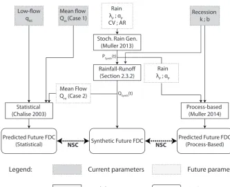
Figure 2. Numerical simulation analysis to assess predictions under change. Future rainfall characteristics (frequencyλP, mean intensity
αP, auto-correlation coefficient AR and coefficient of variation CV) are determined according to expected changes in rain regimes in Nepal
(see Sect. 2.3.2) and fed into a stochastic rainfall generator. The resulting 1000 years of synthetic daily rainfall values (PSynth(t )) are fed
into a rainfall–runoff model that simulates the processes described in Sect. 2.1.1. The rainfall–runoff model uses current recession, soil, and evapotranspiration conditions observed at the Chepe Kohla catchment. The resulting 1000 years of synthetic daily flow values (QSynth(t ))
are then reordered to construct an empirical synthetic (future) FDC, which was compared (in terms of the Nash–Sutcliffe coefficient) to modeled FDCs predicted by the statistical and process-based models. The process-based model admits current recession conditions but
future estimates for rainfall frequency (λP) and mean intensity (αP). Note that unlike the numerically generated empirical FDC, the
process-based model assumes Poissonian rainfall with exponentially distributed depths, that is, CV=1 and AR=0. Current low-flow characteristics (q95) are fed into the statistical model, as well as the current or future (i.e., computed from synthetic streamflow time series) mean flow,
depending on the extent to which mean rainfall is an unbiased predictor of mean flow (Cases 1 and 2 described in Sect. 2.3.2).
records on parameter estimation, and propagated the ensuing uncertainty in the parameters to the FDCs predicted by each model. To do this, we selected a fixed number of full years of streamflow observations, estimated the parameters, predicted the FDC using these parameters, and compared the results to the empirical FDC obtained from the full observation record. The procedure was repeated 10 000 times. The estimation er-rors in the model parameters and the resulting FDC predic-tion performances (NSC) were recorded as a funcpredic-tion of the number of sampled years. This analysis is not intended to de-scribe the models’ ability to predict FDCs at catchments with short observation records: in this case, constructing an em-pirical FDC using the available (however short) observation record is likely to be the best course of action (Castellarin et al., 2004a). Instead, the analysis is intended to simulate the effect of short observation records on FDC prediction at nearby, ungauged catchments. The underlying assumptions behind this analysis are that (i) the error associated with
inter-polation is independent of the flow record length, and (ii) the Chepe Kohla catchment is representative of Nepalese basins. 2.3.2 Predictions under change
We used numerical simulations to assess the ability of both models to predict streamflow when subject to changing rain-fall regimes, as described in Fig. 2.
syn-1 10 100 1000
3/s]
Obs. Sim. Sim (Future)
0.0 0.2 0.4 0.6 0.8 1.0
Duration [−] 0.5 0.6 0.7 0.8 0.9 1.0 1.1
0.80
0.90
1.00
NSC/NSC0
λP
/λP,0 α
P/αP,0
1.25 1.25 1 0.75
Year 1986 10 20 30
0
Observed Predicted
1988 1990 1992 3/s]
[image:8.612.125.469.66.173.2](a) (b) (c)
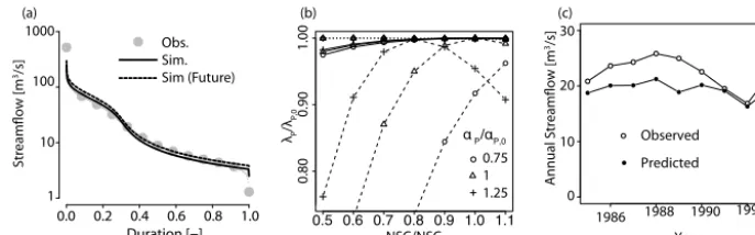
Figure 3. Sensitivity of models to changes in the precipitation regime. (a) Empirical and simulated flow duration curves at Chepe Kohla. The simulated FDC obtained from the stochastic rainfall generator and the bucket watershed model (solid) reproduce the empirical FDC constructed from the observed streamflow well (grey dots). Rainfall changes expected in Nepal (αP/αP,0=1.2,λP/λP,0=0.98) do not have
a substantial influence on the simulated flow distribution (dashed).αPandλPdesignate the mean depth and frequency of wet-season rainfall,
respectively. (b) Sensitivities to relative changes in rainfall frequency and intensity over the Chepe Kohla catchment. The performance of the process-based model is not affected by rainfall changes (dotted). The sensitivity of the statistical model depends on its ability to predict changes in mean flow from annual rainfall. The model is highly sensitive to rain changes if average streamflow cannot be predicted (dashed), and is robust to moderate changes if average flow is perfectly predicted (solid). (c) The linear regression of the statistical model underestimates annual flows at the Chepe Kohla when using a cross-sectional sample (25 gauges) to estimate the local relation between average rainfall and average runoff.
thetic rainfall into a linear reservoir (with a recession con-stant k) with linear evapotranspiration losses, as in Müller et al. (2014). Dry-season discharge was obtained by simulat-ing non-linear seasonal recessions of durationTdstarting at randomly selected runoff peaks in the (previously generated) wet-season streamflow. These assumptions are close to the observed reality in Nepal, as seen in Fig. 3a, where the FDC constructed from the simulated streamflow is a close approx-imation to the empirical FDC in the Chepe Kohla watershed. We translated the effect of shifts in precipitation regimes into changed streamflow for the Chepe Kohla catchment by con-sidering a range of future combinations for rainfall frequen-cies and intensities. In line with what is expected in Nepal (Turner and Slingo, 2009; Turner and Annamalai, 2012), we considered negative changes in the frequency and posi-tive changes in the mean daily rainfall depth. We neglected changes in soil moisture capacity, evapotranspiration, rainfall autocorrelation, and the duration of the rainy season. These parameters are explicit in the process-based model, so we expect differences in the sensitivity of the process-based and statistical models to climate change to be underestimated by this procedure. For each rainfall scenario, we evaluated the performance of the models in a changing climate by gen-erating 1000 years of daily streamflow using future rainfall frequencies and intensities.
We compared the synthetic FDCs to model predictions that were made with future rainfall statistics but
contempo-rary recession and low-flow parameters (Fig. 2). The
statis-tical method in Chalise et al. (2003) uses a linear regression over a cross-sectional sample of observations to predict mean flow based on mean rainfall and altitude. The regression may fail to capture a variety of unobserved characteristics affect-ing both rainfall and streamflow (e.g., local topographic
fea-tures), and hence may not capture the causal relation between the two variables. The extent of this bias cannot be quanti-fied a priori, so we considered two extreme cases: infinite and zero bias. The infinite bias case (Case 1 in Fig. 2) rep-resents the case where no effective relationship can be de-termined between rainfall and mean flow. The best estimator of future mean flow is then the current flow condition. Con-versely, if regression coefficients perfectly describe the effect of annual rainfall on average flow (Case 2 in Fig. 2), then the future flow conditions can be perfectly estimated using the (known) future annual rainfall. We modeled this situation by estimatingQm directly from the (simulated) future flow conditions. While the two cases differed in the determination of mean flow (Qm), the low-flow parameter (q95) was deter-mined from current flow conditions in both cases. In Chalise et al. (2003),q95is normalized byQmand represents reces-sion behavior, which is assumed independent of rainfall. The process-based predictions were obtained by inserting future rainfall statistics and contemporary recession constants into the analytical FDC equation described in Appendix A. The two models were compared by plotting prediction perfor-mances (NSC) against the relative change in the frequency and intensity of synthetic rainfall.
0.0 0.2 0.4 0.6 0.8 1.0
0.25
0.5
1
2
4
Median 50% CI 80% CI
0.0 0.2 0.4 0.6 0.8 1.0 0.6 0.8 1.0
Process Stat.
(a) (b) (c)
QPr
ed
/QObs
Process-based Model Statistical Model Nash–Sutcliffe coefficient
(Log Q)
[image:9.612.131.468.68.197.2]Duration [-]
Figure 4. Flow duration curve prediction performance in ungauged basins. The error duration curves of the leave-one-out cross-validation analysis using the process-based and statistical models are presented in panels (a) and (b), respectively. Relative errors are plotted on a log scale in order to allow the graphs to be balanced on theyaxis: a relative prediction error of 2 (the model predicts double the observed value) is at the same distance fromy=1 (perfect prediction) as a relative error of 1/2 (the model predicts half the observed value). Durations are plotted on thexaxis, withx=0 andx=1 for the highest and lowest flow quantiles, respectively. Panel (c) shows box plots of Nash–Sutcliffe coefficients computed from log-transformed flow quantiles.
Lastly and most importantly, empirical observations reveal that synthetic streamflow distributions generated under con-temporaneous rainfall conditions reproduce closely FDCs constructed from gauge records (Fig. 3a), showing that the underlying recession assumptions are, in fact, representative of runoff processes actually occurring in Nepal.
3 Results
3.1 Prediction in ungauged basins
Results from the leave-one-out cross-validation analysis are presented in Fig. 4 and show that both methods perform sim-ilarly in the prediction of FDCs in ungauged basins. Error duration curves (Fig. 4a and b) show comparable streamflow prediction uncertainties: 75 % of the predicted flow quantiles are between half and double the observed streamflow for both models, although the low flows in the process-based model display an increasing upwards bias (Fig. 4b). Considering the Nash–Sutcliffe coefficients computed at the individual basin level, the mean and median performances are again com-parable for both models, but the accuracy of the statistical model predictions is more variable across sites than the pro-cess model predictions, as indicated by the larger spread of the Nash–Sutcliffe coefficients (Fig. 4c).
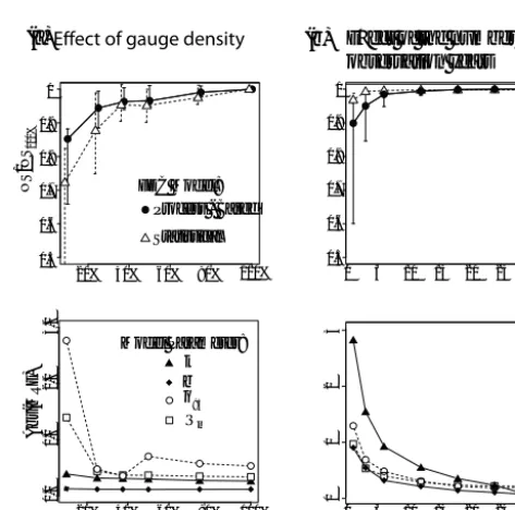
Figure 5a (top) shows prediction performances of both models as the number of streamflow gauges available for predictions decreases, and indicates that the performance of both models is relatively insensitive to the gauge density, until it declines to less than approximately 0.6 gauges per 10 000 km2. For such situations, which represent discarding of more than half the available gauges in Nepal, the statis-tical model performance declines rapidly compared to the process-based model. Prediction performances are strongly affected by uncertainties on the interpolation of model
pa-NS/NS
100%
20% 40% 60% 80% 100%
0.5 0.6 0.7 0.8 0.9 1
Process - Based Statistical
0.0
1.0
2.0
3.0
Ratio of Sampled Gauges
20% 40% 60% 80% 100%
FDC Model:
(a)
0 5 10 15 20 25 30
0.5 0.6 0.7 0.8 0.9 1
0
1
2
3
0 5 10 15 20 25 30
Observation years
(b)
Abs(MRE)
q95 Qm Model Parameter:
k b
Effect of the number of observation years
[image:9.612.311.548.314.548.2]rameters, as seen in Fig. 5a (bottom). Interpolation uncer-tainties are generally larger for the flow indices of the sta-tistical model (Qm andq95) than for the recession param-eters of the process-based model (k and b). This explains the larger spread in prediction performances of the former (Fig. 4c and error bars in Fig. 5a (top)). The parameter un-certainties are also relatively insensitive to the total gauge density until about 60 % of the originally available gauges are discarded. At this point, the uncertainties associated with estimation of the flow indices increase significantly, while the process-based model parameters remain more reasonably es-timated.
When considering short observation windows, parameter uncertainties also drive the performance of the models. Fig-ure 5b (top) shows the prediction performance of both mod-els at the Chepe Khola watershed, as the number of observa-tion years used to estimate the model parameters is reduced. In this case, the statistical model outperforms the process-based model when less than 10 years of streamflow obser-vations are available. The parameter uncertainties associated with the short time-series estimates (Fig. 5b, bottom) suggest that a longer time series of streamflow observations is needed to accurately estimate the wet-season recession parameter (k), resulting in the lower performance of the process-based model for short streamflow records.
3.2 Prediction under change
Simulation results presented in Fig. 3b show both models’ ability to predict a simulated future flow duration curve of the Chepe River under a range of different possible changes in rainfall regimes. In all simulations, parameters describing the hydrological response of the basin (k,b, andq95) are deter-mined using current flow conditions, and evapotranspiration is assumed constant. The results show that explicitly model-ing rainfall–runoff processes allows the process-based model to accommodate the effects of the changing precipitation regime. In contrast, the performance of the statistical model is affected to various degrees by shifts in rainfall regimes, de-pending on how the model translates changes in annual pre-cipitation to changes in average flows. If these shifts are per-fectly represented by the model, then prediction errors arise solely from changes in the shape of the FDC, and the pro-cess and statistical models perform similarly in the Chepe Kohla watershed across the full range of considered rainfall scenarios (Fig. 3b, dashed curve). If, however, average (fu-ture) streamflows cannot be reliably predicted from the pre-dicted changes in annual rainfall, the statistical model does not accommodate flow regime changes at all. In this case, future FDCs are modeled using current streamflow observa-tions, and the ensuing prediction errors can be substantial (Fig. 3b, dotted curve). The simulated cases provide upper and lower bounds for the actual performance of the statistical model in future rainfall regimes. We evaluated the model’s ability to predictQmby using cross-sectional data (i.e.,
aver-age streamflow and annual rainfall from the 25 catchments) to estimate the linear relation betweenQmand annual rainfall Ry. Applied to the Chepe Kohla watershed, the estimated re-gression coefficients allowed the annual streamflow to be es-timated from annual precipitation with a bias of−13 % and a coefficient of determination ofR2=0.57 (Fig. 3c). Regard-less, prediction errors remained negligible for both bounds (NSC>0.95) for the range of changes actually anticipated in Nepal (e.g.,1λP/λP≈0.98 and1αP/αP≈1.20 for the 2·CO2scenario – Turner and Slingo, 2009).
4 Discussion
4.1 Predictions in ungauged basins
The analysis suggests that both statistical and process-based methods to estimate FDCs in ungauged basins perform com-parably in Nepal, over a wide range of gauge densities and observation durations. Yet prediction performances varied significantly between the models as data became increas-ingly sparse. The statistical method is more sensitive to spa-tially sparse data, which degrades the interpolation accuracy ofQm. In contrast, the estimation method for recession pa-rameters makes the process-based approach more sensitive to temporally restricted observations, which reduce the accu-racy with which recession parameters can be estimated. This suggests that the performance of the two models in ungauged basins is affected by different sources of uncertainty. In this section, we investigate the source of prediction error in each method and discuss the implications for their application in ungauged basins beyond Nepal.
4.1.1 Sources of uncertainty
The statistical model relies on two assumptions about the correlations of observed data. The first assumption is that catchments with similar low-flow indices (q95) have identical hydrological responses, and therefore identical FDC shapes. Second, the model assumes that the flow indices (Qm and q95) at ungauged catchments can be best predicted using lin-ear regressions against observable covariates (annual rain-fall, elevation, and geology). The latter assumption does not hold if the flow indices are spatially auto-correlated, or if the posited linear relations are spatially heterogeneous or, in fact, non-linear. Furthermore, “omitted variable” biases (Greene, 2003) will arise if an unobserved variable is correlated with both a covariate and a flow index. For instance, local topo-graphic features may affect both the annual rainfall and the average streamflow in mountainous regions. Violation of the second assumption leads to substantial uncertainty in the in-terpolation of the flow indices in Nepal and drives the predic-tion errors of the statistical approach, as shown in Sect. S2 of the Supplement.
arise from simplifying assumptions about local hydrologi-cal processes (rather than uncertainties from their statistihydrologi-cal interpolation from neighboring gauges). Additional cross-validation analyses (shown in Sect. S2 of the Supplement) suggest that uncertainties caused by the aggregation of ob-served point-rainfall statistics at the catchment level drive prediction errors of high-flow quantiles. While increasingly accurate remote sensing rainfall data will progressively al-low such spatial heterogeneities to be resolved, current pre-cipitation products (e.g., TRMM 3B42) remain substantially biased in mountainous regions like Nepal, where they do not outperform available rain gauges in predicting the frequency and intensity of areal rainfall (Müller and Thompson, 2013). A second source of error arises from the simplifying assump-tions made about streamflow recession that do not hold per-fectly in the observed catchments. Because they describe the same watershed, the wet and dry recession parameters are assumed to be physically related. In Müller et al. (2014), the scale parameter of the non-linear seasonal recession (a) is expressed as an explicit function of the two recession param-eters (kandb) for sufficiently short recession times, where power-law recessions can be approximated by exponential functions. We show in the Supplement (Sect. S2) that, al-though this approach provides more accurate estimates ofa than would be obtained through spatial interpolation, estima-tion uncertainties remain, propagate through the model, and result in prediction errors during the dry season.
4.1.2 Applicability beyond Nepal
This study compares two specific methods on their ability to predict FDCs in the particular context of ungauged Nepalese basins. Results are thus not necessarily representative of the relative performance of process-based and statistical meth-ods in general, particularly in regions where abundant field data allow more advanced statistical approaches to be im-plemented. Yet fundamentally, the statistical model relies on observed correlations rather than assumptions about hydro-logic mechanisms. Because FDC shapes are modeled non-parametrically, the approach is applicable to regions with highly variable catchment responses. However, prediction performance in ungauged basins is constrained by interpo-lation errors in the mean flow. This makes the method un-suitable for regions where the local determinants of mean flow (i.e., rainfall, evapotranspiration, glacial melt) cannot be accurately monitored at the catchment level. In contrast, a key advantage of the process-based model is its ability to ex-ploit characteristics of the stochastic structure of rainfall that can be estimated from daily rainfall observations. The model is appropriate for regions where the spatial heterogeneity of runoff is driven by rainfall, and where the frequency and in-tensity of rainfall depths at the catchment level can be readily estimated (i.e., small catchments with numerous rain gauges, or places where satellite observations provide a good rep-resentation of rainfall statistics). Unlike rainfall, recession
behavior arises from lumped and complex interactions be-tween climate, vegetation, and groundwater processes that typically cannot be monitored in a spatially explicit manner. The process-based model is therefore inappropriate for re-gions where the hydrologic response of the catchment is the main source of runoff heterogeneity, or where the assumed recession behavior (in particular the relation between a,k, andb) does not occur.
Conveniently, the appropriate implementation contexts for both methods appear to be complementary, and the optimal method in a given region is determined by the driving source of runoff heterogeneity in the catchments. Ultimately, the performance of both methods is constrained by their abil-ity to estimate their parameters in ungauged basins. This re-lation is apparent in Fig. 5, where drops in prediction per-formances correspond to increases in the estimation uncer-tainty of model parameters. Under these conditions, the per-formance of each method is driven by the ability of the avail-able observations to capture the variability of the model pa-rameters. When interpolated from neighboring gauges, un-certainties are governed by the interplay between the layout of the gauges and the spatial correlation range of the consid-ered model parameter. When estimated from short observa-tion records, accuracy is determined by the extent to which the available record is representative of the temporal variabil-ity of the parameter. These interactions between data avail-ability and runoff variavail-ability are inherently local and will af-fect the determination of the most appropriate method for any given region.
4.2 Prediction under change
In contrast, the statistical model is solely based on ob-served correlations, leading to two important sources of er-rors for predictions under change. First, the model only ac-commodates rainfall changes to the extent that the estimated statistical relation between rainfall and runoff is representa-tive of local runoff coefficients. The model will not reliably predict future streamflows if runoff coefficients are strongly spatially heterogeneous, or if the cross-sectional sample of gauges fails to capture important processes governing mean flow. This source of uncertainty appears to be significant in Nepal, as illustrated by the substantial bias in annual flow predictions in Fig. 3c. Secondly, the statistical model only considers the effect of average rainfall on average flow: the effect of rainfall distribution on streamflow distribution is ignored. As a result, the model cannot predict changes in the shape of FDCs that are brought about by changing rain-fall. The prediction performance of the statistical approach is therefore determined by the resilience of the flow regime, that is, the extent to which streamflow distribution is affected by shifting rain signals (Botter et al., 2013): the method will perform poorly in catchments with non-resilient flow regimes. The Monte Carlo analysis presented in the Supple-ment (Sects. S3 and S4) shows that streamflow resilience in seasonally dry catchments depends on two distinct seasonal effects: a “direct” effect driven by the ratio betweenλPandk during the wet season, and an “indirect” effect during the dry season, when resilience is determined by the interplay be-tweenQ0(i.e., wet-season rainfall) andb. In seasonally dry climates, we expect the statistical method to be most reli-able in regions where wet seasons are short with limited total rainfall but persistent flow regimes, and where the recession behavior during the dry season is close to linear.
Lastly, a key assumption in this study is that catchment response (in terms of low-flow or recession characteristics) is independent of climate. It is possible that shifts in climate have an effect on catchment response by affecting the parti-tioning of effective rainfall between storage and runoff. Al-though not quantitatively assessed in this study, we expect that this effect would negatively affect the performance of both approaches.
5 Conclusions
Stochastic, process-based models predicted the FDCs for un-gauged catchments in Nepal well, with a performance that was comparable to that of statistical models. It suggests that in regions with globally representative gauge densities, and under seasonally dry climates, the advantages of the statis-tical approaches relative to stochastic models noted in pre-vious analyses (Blöschl et al., 2013) may not apply. Funda-mentally, the performances of both approaches are strongly affected by the method chosen to estimate model parameters in ungauged basins, so this conclusion comes with the caveat that this study cannot be interpreted as a general benchmark
to compare these approaches at a global level. Although we believe that the selected models are appropriate to compare process-based and statistical approaches for practical PUB application in Nepal, their relative performance may be dif-ferent in other regions, where more abundant information on catchment characteristics allow more complex (and presum-ably more accurate) regionalization approaches to be applied. Thus, substantial research remains to be done to compare these approaches in other parts of the world, where locally appropriate methods should be carefully considered.
Nonetheless, this study finds a complementarity between the different sources of uncertainty in the stochastic and sta-tistical methods. This suggests that model selection should be driven by a consideration of the main drivers of heterogeneity in any study catchment: process-based models are advisable if climate is likely to be the main source of runoff hetero-geneity. Conversely, statistical methods are more appropriate for regions with substantially different recession behaviors across catchments. These distinctions provide a potentially robust basis for model selection in any given application.
The results also suggest that the sensitivity of statistical approaches to changes in rainfall statistics is dependent on the “resilience” of the flow regime as defined by Botter et al. (2013). Overall, the process-based models are more reliable in projecting FDCs into new rainfall regimes. This is par-ticularly true for catchments characterized by a strong wet-season runoff and a rapid, strongly non-linear hydrologic re-sponse, because their flow regime is particularly vulnerable to rainfall changes, making the assumptions of the statistical model inappropriate.
Appendix A: Process-based streamflow distribution model for seasonally dry climates
This appendix presents the analytical expression of FDC in seasonal climates derived in Müller et al. (2014). The approach assumes that rainfall can be represented as a marked Poisson process with exponentially distributed depths. Catchments are modeled as spatially homogenous linear reservoirs with linear evapotranspiration losses. Un-der these conditions, wet-season streamflow can be repre-sented as a gamma-distributed random variable (Botter et al., 2007b):
Qw∼0(m, αQ−1),
withm=λ/ kandαQ=αPkA, and wherekis the linear
re-cession constant, A the area of the contributing catchment and αP the mean intensity of wet-season rainfall. The fre-quency λ of runoff events can be expressed as a function of the frequency (λP) and intensity of rainfall (Botter et al., 2007b):
λ=ηexp(−γ )γ
λP η
0L(λP/η, γ )
, (A1)
where0L(·,·)is the lower incomplete gamma function, and where η=ET/SSC andγ =SSC/αP are, respectively, the ratio between maximum evapotranspiration and soil storage capacity, and the ratio between soil storage capacity and mean rainfall intensity.
Dry-season streamflow is modeled as a seasonal reces-sion starting at the last discharge peak of the wet season. Because wet-season streamflow is a gamma-distributed vari-able, streamflow at discharge peaks, and therefore the ini-tial condition of the seasonal recession, is itself a gamma-distributed variable (Müller et al., 2014):
Qpeak∼0(m+1, αQ−1).
Assuming a power-law relation between discharge and recession rate, the cumulative distribution function of dry-season streamflow can be expressed as (Müller et al., 2014)
PQd(Q)=
1+q r
d01−αrQ02
arTd0(m+1), ifQ >−(arTd) 1
r
andr <0 1+q
r
d01−αrQ02
arTd0(m+1) otherwise
+α r
Q04+(Qr−arTd)03 arTd0(m+1) , with
01 = 0U(m+1, αQ−1Q),
02 = 0U
r+m+1, αQ−1Q
,
03 = 0U
m+1, α−Q1(Qr+arTd)1r
,
04 = 0U
r+m+1, αQ−1(Qr+arTd) 1
r
.
0(·) and 0U(·,·) denote the complete and upper incom-plete gamma functions;Tdis the duration of the dry season; r=1−b anda are the parameters of the non-linear reces-sion, which are assumed stationary. Because they describe the same watershed, recession parameters for the wet and dry seasons are related. If power-law recessions can be ap-proximated by an exponential function for sufficiently short recession times, we can expressa as a function ofk andb (Müller et al., 2014):
a≈ λ −r
e−mr −1 αQ·(m+1). (A2)
The law of total probability can finally be used to combine seasonal streamflow distributions and derive the cumulative distribution function of streamflow for the whole year: PQ(Q)=
1− Td
365
·PQw(Q)+ Td
365·PQd(Q). (A3) The FDC for seasonally dry climates is finally obtained by plotting the streamflow quantilesQagainst 1−PQ(Q),
The Supplement related to this article is available online at doi:10.5194/hess-20-669-2016-supplement.
Acknowledgements. The Swiss National Science Foundation is gratefully acknowledged for funding (M. F. Müller).
Edited by: S. Archfield
References
Alaouze, C. M.: Reservoir releases to uses with different reliability requirements, AWRA Water Resour. Bull., 25, 1163–1168, 1989. Alternative Energy Promotion Center: Construction and Installation Manual for Micro Hydropower Project Installers, Government of Nepal, 2014 (in Nepalese).
Arora, M., Goel, N., Singh, P., and Singh, R.: Regional flow du-ration curve for a Himalayan river Chenab, Nord. Hydrol., 36, 193–206, 2005.
Basso, S. and Botter, G.: Streamflow variability and optimal capac-ity of run-of-river hydropower plants, Water Resour. Res., 48, W10527, doi:10.1029/2012WR012017, 2012.
Bélisle, C. J.: Convergence theorems for a class of simulated an-nealing algorithms on Rd, J. Appl. Probab., 29, 885–895, 1992. Blöschl, G., Sivapalan, M., Wagener, T., Viglione, A., and
Savenije, H.: Runoff Prediction in Ungauged Basins: Synthesis across Processes, Places and Scales, Cambridge University Press, 2013.
Botter, G., Peratoner, F., Porporato, A., Rodriguez-Iturbe, I., and Rinaldo, A.: Signatures of large-scale soil moisture dynamics on streamflow statistics across U.S. climate regimes, Water Resour. Res., 43, W11413, doi:10.1029/2007WR006162, 2007a. Botter, G., Porporato, A., Rodriguez-Iturbe, I., and Rinaldo, A.:
Basin-scale soil moisture dynamics and the probabilistic charac-terization of carrier hydrologic flows: slow, leachingprone com-ponents of the hydrologic response, Water Resour. Res., 43, W02417, doi:10.1029/2006WR005043, 2007b.
Botter, G., Porporato, A., Rodriguez-Iturbe, I., and Ri-naldo, A.: Nonlinear storage–discharge relations and catch-ment streamflow regimes, Water Resour. Res., 45, W10427, doi:10.1029/2008WR007658, 2009.
Botter, G., Basso, S., Rodriguez-Iturbe, I., and Rinaldo, A.: Re-silience of river flow regimes, P. Natl. Acad. Sci. USA, 110, 12925–12930, doi:10.1073/pnas.1311920110, 2013.
Brutsaert, W. and Nieber, J. L.: Regionalized drought flow hydro-graphs from a mature glaciated plateau, Water Resour. Res., 13, 637–643, doi:10.1029/WR013i003p00637, 1977.
Castellarin, A., Galeati, G., Brandimarte, L., Montanari, A., and Brath, A.: Regional flow-duration curves: reliability for ungauged basins, Adv. Water Resour., 27, 953–965, doi:10.1016/j.advwatres.2004.08.005, 2004a.
Castellarin, A., Vogel, R., and Brath, A.: A stochastic index flow model of flow duration curves, Water Resour. Res., 40, W03104, doi:10.1029/2003WR002524, 2004b.
Castellarin, A., Botter, G., Hughes, D., Liu, S., Ouarda, T., Para-jka, J., Post, D., Sivapalan, M., Spence, C., Viglione, A., and Vo-gel, R.: Prediction of flow duration curves in ungauged basins,
chapt. 7, in: Runoff Prediction in Ungauged Basins: Synthesis Across Processes, Places and Scales, edited by: Blöschl, G., Siva-palan, M., Wagener, T., Viglione, A., and Savenije, H., Cam-bridge University Press, 135–162, 2013.
Ceola, S., Botter, G., Bertuzzo, E., Porporato, A., Rodriguez-Iturbe, I., and Rinaldo, A.: Comparative study of ecohydrolog-ical streamflow probability distributions, Water Resour. Res., 46, W09502, doi:10.1029/2010WR009102, 2010.
Chalise, S., Kansakar, S., Rees, G., Croker, K., and Zaidman, M.: Management of water resources and low flow estimation for the Himalayan basins of Nepal, J. Hydrol., 282, 25–35, doi:10.1016/S0022-1694(03)00250-6, 2003.
Cheng, L., Yaeger, M., Viglione, A., Coopersmith, E., Ye, S., and Sivapalan, M.: Exploring the physical controls of re-gional patterns of flow duration curves –Part 1: Insights from statistical analyses, Hydrol. Earth Syst. Sci., 16, 4435–4446, doi:10.5194/hess-16-4435-2012, 2012.
Chitrakar, P.: Micro-Hydropower Design Aids Manual, Small Hy-dropower Promotion Project (GTZ) and Mini-Grid Support Program, Alternate Energy Promotion Center, Government of Nepal, 2004.
Coopersmith, E., Yaeger, M. A., Ye, S., Cheng, L., and Siva-palan, M.: Exploring the physical controls of regional patterns of flow duration curves – Part 3: A catchment classification sys-tem based on regime curve indicators, Hydrol. Earth Syst. Sci., 16, 4467–4482, doi:10.5194/hess-16-4467-2012, 2012. Department of Hydrology and Meteorology: Daily Streamflow and
Precipitation Data, Kathmandu, 2011.
Doulatyari, B., Betterle, A., Basso, S., Biswal, B., Schirmer, M., and Botter, G.: Predicting streamflow distributions and flow duration curves from landscape and climate, Adv. Water Resour., 83, 285– 298, doi:10.1016/j.advwatres.2015.06.013, 2015.
Dralle, D. N., Karst, N., and Thompson, S.: Dry season stream-flow persistence in seasonal climates, Water Resour. Res., doi:10.1002/2015WR017752, online first, 2015.
Global Runoff Data Center: Global Runoff Data Base, Global Runoff Data Centre, Koblenz, Federal Institute of Hydrology (BfG), 2014.
Greene, W. H.: Econometric Analysis, Prentice Hall, Upper Saddle River, NJ, 2003.
HKH-FRIEND: Hindu Kush Himalayan – Flow Regimes from In-ternational Experimental and Network Data, UNESCO Interna-tional Hydrological Programme, UNESCO Paris, France, 2004. Hughes, D. and Smakhtin, V.: Daily flow time series patching or
ex-tension: a spatial interpolation approach based on flow duration curves, Hydrol. Sci. J., 41, 851–871, 1996.
Lambert, L. and Chitrakar, B.: Variation of potential evapotranspi-ration with elevation in Nepal, Mt. Res. Dev., 9, 145–152, 1989. Lazzaro, G., Basso, S., Schirmer, M., and Botter, G.: Water man-agement strategies for run-of-river power plants: profitability and hydrologic impact between the intake and the outflow, Water Re-sour. Res., 49, 8285–8298, doi:10.1002/2013WR014210, 2013. Milly, P., Julio, B., Malin, F., Robert, M., Zbigniew, W.,
Den-nis, P., and Ronald, J.: Stationarity is dead, Science, 319, 573– 574, doi:10.1126/science.1151915, 2008.
Decade 2013–2022, Hydrolog. Sci. J., 58, 1256–1275, doi:10.1080/02626667.2013.809088, 2013.
Mu, X., Zhang, L., McVicar, T. R., Chille, B., and Gau, P.: Analysis of the impact of conservation measures on stream flow regime in catchments of the Loess Plateau, China, Hydrol. Process., 21, 2124–2134, doi:10.1002/hyp.6391, 2007.
Müller, M. F.: Bridging the Information Gap: Remote Sensing and Micro Hydropower Feasibility in Data-Scarce Regions, Doctoral Dissertation, University of California, Berkeley, CA, 2015. Müller, M. F. and Thompson, S. E.: Bias adjustment of satellite
rainfall data through stochastic modeling: methods development and application to Nepal, Adv. Water Resour., 60, 121–134, doi:10.1016/j.advwatres.2013.08.004, 2013.
Müller, M. F. and Thompson, S. E.: TopREML: a topological re-stricted maximum likelihood approach to regionalize trended runoff signatures in stream networks, Hydrol. Earth Syst. Sci., 19, 2925–2942, doi:10.5194/hess-19-2925-2015, 2015. Müller, M. F., Dralle, D. N., and Thompson, S. E.: Analytical model
for flow duration curves in seasonally dry climates, Water Re-sour. Res., 50, 5510–5531, doi:10.1002/2014WR015301, 2014. Muneepeerakul, R., Azaele, S., Botter, G., Rinaldo, A., and
Rodriguez-Iturbe, I.: Daily streamflow analysis based on a two-scaled gamma pulse model, Water Resour. Res., 46, W11546, doi:10.1029/2010WR009286, 2010.
NASA Land Processes Distributed Active Archive Center (LP DAAC): ASTER GDEM v2, NASA Land Processes Distributed Active Archive Center (LP DAAC), ASTER L1 B, USGS/Earth Resources Observation and Science (EROS) Center, Sioux Falls, 2011.
Nathan, R. and McMahon, T.: Evaluation of automated techniques for base flow and recession analyses, Water Resour. Res., 26, 1465–1473, 1990.
Sauquet, E. and Catalogne, C.: Comparison of catchment group-ing methods for flow duration curve estimation at ungauged sites in France, Hydrol. Earth Syst. Sci., 15, 2421–2435, doi:10.5194/hess-15-2421-2011, 2011.
Schaefli, B., Rinaldo, A., and Botter, G.: Analytic probability distri-butions for snow-dominated streamflow, Water Resour. Res., 49, 2701–2713, doi:10.1002/wrcr.20234, 2013.
Searcy, J. and Hardison, C.: Double-Mass Curves. Manual of Hy-drology: Part I, General Surface Water Techniques, US Geolog-ical Survey Water-Supply Paper 1541-B, United States Govern-ment Printing Office, Washington, 1960.
Shao, J. and Tu, D.: The Jackknife and Bootstrap, Springer-Verlag, New York, 2012.
Shrestha, D. P.: Assessment of soil erosion in the Nepalese Hi-malaya: a case study in Likhu Khola Valley, Middle Mountain Region, Land Husbandry, 2, 59–80, 1997.
Stokstad, E.: Scarcity of rain, stream gages threatens forecasts, Science, 285, 1199–1200, doi:10.1126/science.285.5431.1199, 1999.
Thompson, S., Levin, S., and Rodriguez-Iturbe, I.: Linking plant disease risk and precipitation drivers: a dynamical systems framework, Am. Nat., 181, E1–E16, doi:10.1086/668572, 2013a. Thompson, S. E., Sivapalan, M., Harman, C. J., Srinivasan, V., Hipsey, M. R., Reed, P., Montanari, A., and Blöschl, G.: De-veloping predictive insight into changing water systems: use-inspired hydrologic science for the Anthropocene, Hydrol. Earth Syst. Sci., 17, 5013–5039, doi:10.5194/hess-17-5013-2013, 2013b.
Turner, A. G. and Annamalai, H.: Climate change and the south Asian summer monsoon, Nature Climate Change, 2, 587–595, doi:10.1038/nclimate1495, 2012.
Turner, A. G. and Slingo, J. M.: Subseasonal extremes of precip-itation and active-break cycles of the Indian summer monsoon in a climate-change scenario, Q. J. Roy. Meteor. Soc., 135, 549– 567, 2009.
United States Geological Survey: USGS Threatened and Endan-gered Streamgages, available at: http://streamstats09.cr.usgs.gov/ ThreatenedGages/ThreatenedGages_str.html (last access: 5 Au-gust 2015), 2015.
Vogel, R. and Fennessey, N.: Flow-duration curves. I: New inter-pretation and confidence intervals, J. Water Res. Pl.-ASCE, 120, 485–504, 1994.