e
-ISSN: 2278-067X,
p
-ISSN : 2278-800X, www.ijerd.com
Volume 5, Issue 7 (January 2013), PP. 75-83
Comparative Performance of Linear and CG Based
Partitioning Of Histogram for Bins Formation in CBIR
Dr. H. B. Kekre
1, Kavita Sonawane
21Sr. Professor /Department of Computer Engineering, MPSTME, NMIMS University, Mumbai, India 2Ph.D Research Scholar/Department of Computer Engineering, MPSTME, NMIMS University Mumbai, India
Abstract:- This paper presents the CBIR based on bins approach. It introduces a new idea of
partitioning the histogram into three parts using Centre of gravity. This partitioning leads to generation of 27 bins. In this work we have tried to reduce the feature vector dimension to just 27 bins out of 256 histogram bins. This paper elaborates the bins approach using linear (LP) and centre of gravity (CG) based histogram partitioning for generation of 27 bins. Image contents extracted to these bins are the count of pixels falling in the specific range of intensities plotted in the R, G and B histograms. These contents are process further by computing the statistical first four moments Mean, Standard deviation, skewness and kurtosis. The moments are computed separately for R, G and B intensities and treated as separate feature vectors and stored in separate feature databases. Experimentation work is carried out using database of 2000 BMP images having 20 classes including few from Wang database. Core part of this CBIR i.e comparison of query and database images is facilitated using three similarity measures namely Euclidean distance(ED), Absolute distance (AD) and Cosine correlation distance (CD). Performance of the proposed CBIR system is evaluated using three parameters Precision Recall Cross over Point (PRCP), Longest String (LS), Length of String to Retrieve all Relevant (LSRR).
Keywords:- CBIR, Bins, Centre of Gravity, Linear Partitioning, Mean, Standard deviation, Skewness,
Kurtosis, Euclidean distance, Absolute distance, cosine correlation distance, Precision recall Cross over Point, Longest String, Length of String to Retrieve all Relevant.
I.
INTRODUCTION
using the 256 bins of histogram for comparing two images here implemented a new idea of partitioning the histogram which leads to reduction of feature vector dimension from 256 bins to 27 bins. This generates the compact feature vector which speeds up the comparison process. Feature extraction begins by separating the image into R, G and B planes. For each plane obtain the histogram which is partitioned into three parts using CG and LP partitioning techniques [21][22][23][24]. This process leads to generation of 27 bins. Information extracted to these 27 bins is the count of pixels falling in the specific intensity range. This information is further processed and four types of feature vectors are computed from it based on the first four absolute moments. Each type of feature with respect to each moment is stored separately. The same feature extraction process is followed for both partitioning techniques and multiple feature vector databases are prepared. Query by example approach is used here to test the system‟s response. Once query enters into the system a feature vector will be extracted for the same and will be compared with all feature vectors of the images in the database. This comparison is carried out using three similarity measures. One is very commonly used in CBIR systems as distance measure i.e Euclidean distance. Along with this we have tried two more measures namely absolute and Cosine correlation distance. We found them performing better in many cases as compared to Euclidean distance. Output of the CBIR systems is the set of images similar to given query. According to user‟s point of view, system should retrieve as many as possible images of query class from large size databases. To check and evaluate the system‟s performance to achieve user‟s satisfaction, we have used three different parameters namely Precision Recall Cross over Point (PRCP), Longest String (LS) and Length of String to Retrieve all Relevant (LSRR)[24][25][26]. Proposed Work done is organized as follows. Section II describes the Feature extraction process; Section III describes the comparison process carried using distance measures. Section IV illustrates the performance evaluation parameters. Results and discussions are presented in section V. Finally conclusive remarks are given in section VI followed by references.
II.
FEATURE
EXTRACTION
Feature extraction and comparison process are core phases for any CBIR system. Feature extraction in our work is based on the bins approach. Mainly discussing the bins formation process which actually leads to the feature vector extraction. This process starts from separating the image into R, G and B planes and obtaining their histograms. Following section explains the histogram and it‟s partitioning using CG and LP.
A. R, G and B Planes with Histograms
Very First step being followed in feature extraction is split the image into R, G and B planes shown as follows in Fig.1 for Barbie image.
Fig.1: Barbie Image with R, G and B Planes
Then we obtained the histograms for each one of them as shown in Fig.2
0 50 100 150 200 250 300 0
100 200 300 400
0 50 100 150 200 250 300 0
100 200 300 400
0 50 100 150 200 250 300 0
100 200 300 400
B. Histogram Partitioning techniques :CG and LP
This work is focusing on the feature vector dimension reduction along with the improvement in the retrieval results. To reduce the time and computational complexity instead of using all 256 bins of histogram as it is, trying to make it compact by reducing the number of bins. Thus forming only 27 bins from three histograms (R, G and B). Bins are not selected randomly from the histogram for feature vector; rather partitioning used to partition the histograms into three parts so that it will lead to generation of 27 bins. Two techniques used for partitioning are LP and CG.
LP partitioning:
It simply divides the histogram into three parts such that each partition will have same number of pixels. Thus for three parts get two grey levels, acting as threshold for the pixels to be counted in specific partition. It calculates the grey level thresholds for image size m x n using eq1.
GL1= (m*n)/3 and GL2= 2(m*n)/3 (1)
Here GL1 and GL2 are the two thresholds obtained for three parts. Grey levels for all three (R, G and B) histograms are calculated using eq1. Here obtained the three sets of threshold as follows for sample Barbie image and its histograms shown in Fig.1 and 2 respectively.
LP partitioning for Fig2. Histograms
RGL1 = 215 RGL2 = 252 GGL1 = 171 GGL2 = 236 BGL1 = 155 BGL2 = 223
Fig3. Shows Green Histogram partitioning using LP at two Grey levels GGL1 = 171 and GGL2= 236.
Similarly we have partitioned the red and Blue
histograms with RGL and BGL 1 and 2 respectively.
Fig.3: Green Histogram with 0,1 and 2 Parts :
LP partitioning
CG Partitioning:
We have first worked with LP where the histogram is divided by just taking the count of pixels into consideration. But one important factor we have missed here is the intensities of the pixels are totally ignored and only count has been taken into account. To solve this issue and without ignoring the pixel intensities this new partitioning is implemented i.e partitioning based on Centre of gravity. As we know CG is the point where surrounding weight is equal. Getting two equal parts using CG is simple by computing CG using eq.2; but getting three uniform partitions cannot be done using the CG formula directly. To facilitate this partitioning here the new logic has been derived to get three partitions having equal moments based on CG and its properties.
n
i i
W
n W n L W
L W L CG
1 ... 2 2 1 1
(2)
Fig.4: Green Histogram with 0, 1 and 2 Parts : CG partitioning
using this CG partitioning technique and obtained the following grey levels for R, G and B histogram as follows :
CG partitioning for Fig2. Histograms
RGL1 = 203 RGL2 = 240
GGL1 = 165 GGL2 = 228
BGL1 = 142 BGL2 = 206
The three partitions obtained using LP and CG techniques are identified as part 0, 1 and 2. Now how it leads bins formation is explained as follows:
C. Bins formation and Count of Pixels
After partitioning, start extracting the features for the image under feature extraction process. Let us, pick up the pixel from the image under process and check its R, G and B intensities.
The partition of the respective histogram it falls assign three flag (either 0,1 or 2) bits for R, G and B (intensity) to that pixel. This three bit flag decides the destination bin for the pixel to be counted. The bin address is actually generated using following equation. It ranges from 000 to 222 i.e. Total 27 bins.
Hence if R, G and B intensities of the pixels are falling in partition 0, 2, 2 respectively then flag for the pixel will be set to „022‟. This generates the bin address 8; means that pixel is falling in bin no 8.
This was about how the bins formation process takes place. Using LP and CG dividing the histogram into three parts generates 27 bins from 000 to 222. Initially these bins are holding the count of pixels based on the specific intensity range they belong to. Sample 27 bins obtained for the barbie image (Fig.1) is shown in following Fig.5. On top of each bin the value shown represents the count of pixels it contains. Few bins showing zero contents, e.g. bin no.8 contains zero, it means there are no such pixels present in the images having flag „022‟.
0 1 2 3 4 5 6 7 8 9 1 0 1 1 1 2 1 3 1 4 1 5 1 6 1 7 1 8 1 9 2 0 2 1 2 2 2 3 2 4 2 5 2 6 2 7 2 8 0
5 00 1 00 0 1 50 0 2 00 0 2 50 0 3 00 0 3 50 0 4 00 0 4 50 0 5 00 0 5 50 0 6 00 0
0 0 3 9
6 1 57
2 4 19
2 0 3
0 8 0 4 2 2 0 0 0 7 8 0
1 8 17
2 2 5 58
9 8
0 1
0 1
1 2 95
3 0 0 4 2 9 4 3 1
Fig.5: Sample of 27 Bins Showing Count of Pixels for Barbie Image
Now instead of considering only the count of pixels as feature vector, a thought of giving significance to the intensity each pixel has, is implemented so that we can have feature vector with strong discrimination ability. To implement this idea, first four absolute moments for the R, G and B intensities of the pixels counted into each bin are computed. Each moment computed is stored separately in respective feature vector database. This way, it forms four types of feature vector databases based on the type of moment. One more variation based on the color content is used i.e four moments are calculated and stored separately for R, G and B colours. In all total 24 feature vector databases are prepared as, 4 moments x 3 colors x 2 partitioning techniques. This was the pre-processing part of the proposed CBIR system
III.
COMPARISON
PROCESS:
SIMILARITY
MEASURES
Once the feature vector databases are prepared for all the database images system is ready to face the query image and then comparison takes place. Feature vector for the query image will be extracted and compared with all the database image feature vectors by means of similarity measure. There are various similarity metrics available to compare two images. Most commonly used similarity metric in the CBIR systems is Euclidean distance [16-19]. Here we have not limited it to Euclidean distance (ED), but also have used two more distance measures along with it , namely Absolute distance (AD) and Cosine Correlation distance (CD) [25][26]. Once the distance will be calculated between query and database image features; it will be sorted in ascending order. Then we have to select the images which are close to query based on the distances sorted (from min to max). Following equations 4, 5 and 6 are representing the distance measures ED, AD and CD respectively
r
g
b
Address
Euclidean Distance
21
n
i
i i
QI FQ FI
D
(4)
Absolute Distance
)
(
1
I n
I QI
FQ
FI
D
(5)
Cosine Correlation Distance
( ) ( ) ( ) ( )
) ( ) (
n Q n Q n D n D
n Q n D
Where D(n) and Q(n) are Database
and Query feature Vectors resp. (6)
IV.
PERFORMANCE
EVALUATION
PARAMETERS
Performance evaluation is compulsory step to be followed after designing and implementing any new system. In CBIR systems, it is essential to check and evaluate the system‟s response and behaviour because of various different user expectations from the CBIR system. By taking these expectations into account we have tried to evaluate our proposed system by means of three parameters namely Precision Recall Cross over Point (PRCP), LS(Longest String), LSRR(Length of String to retrieve all Relevant) and are defined as follows.
A. PRCP
PRCP gives the cross over point of two most commonly used parameters precision and recall defined in equations 7 and 8 respectively. Taking cross over point of precision and recall indicates the idealness of the system in very precise way. PRCP =1 is indication of the ideal CBIR system, whereas PRCP =0 indicates the worst case performance of CBIR.
(7)
(8)
B. Longest String(LS)
It identifies the continuous string of relevant images from sorted set of distances. The maximum continuous string of images is then selected as LS parameter. The distances are sorted in ascending order e.g distance of query with all 2000 database images; this is done separately for each color result i,e R, G and B results. Only one maximum LS have been selected from these three color results set. We also have kept track that the final LS is coming from which color result; and this is one way of checking the role of these three colors in the system.
C. Length of String to Retrieve all Relevant (LSRR)
This parameter works on identifying and analysing the response time of the system to recall all images relevant query from the database. Input for this parameter is same i.e set of images (2000) sorted according to distances sorted in ascending order. It is collecting all images available in the database which are relevant to query image; and here LSRR comes in picture which keeps track that how long the system travels to collect all images. The minimum is the traversal, best is the performance and the long it travels indicates the worst it performs. Minimum LSRR can be defined as the traversal length where all query relevant images are extracted as initial continuous string. As users are interested in minimum LSRR; selecting minimum LSRR among results obtained separately for R, G and B colors. Here also we kept track that which color is performing better among three.
V.
RESULTS
AND
DISCUSSION
Fig.6. Sample Images from 20 classes in Database
Once the query image is fired to the system, query feature vector will be extracted and then it will be compared with all feature vector databases by means of three similarity measures ED, AD and CD. Each of these 200 queries is executed for all three performance evaluation parameters PRCP, LS and LSRR. We have analysed and compared these results with respect to the partitioning CG and LP, R, G, B colors and the distance measures used. Result obtained for each parameter for each type of feature vector based on moments is shown in following tables.
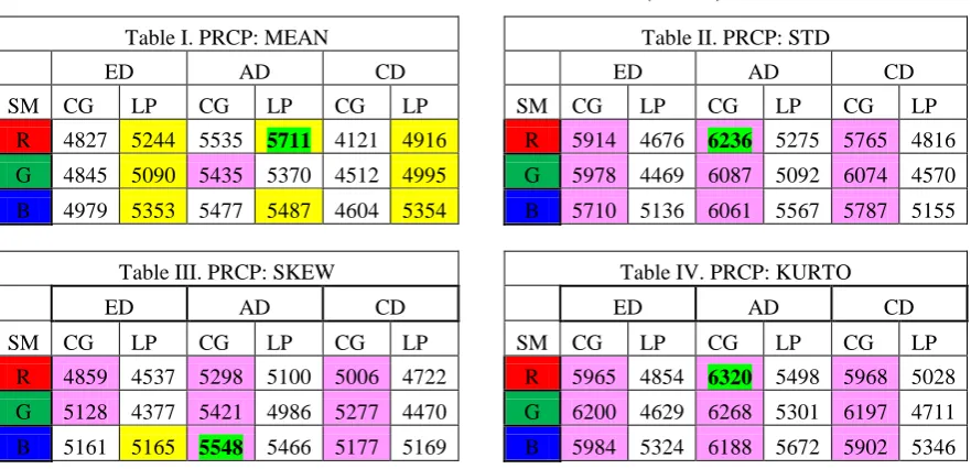
A. Precision Recall Cross Over Point (PRCP )
Table I. PRCP: MEAN
ED AD CD
SM CG LP CG LP CG LP
R 4827 5244 5535 5711 4121 4916
G 4845 5090 5435 5370 4512 4995
B 4979 5353 5477 5487 4604 5354
Table II. PRCP: STD
ED AD CD
SM CG LP CG LP CG LP
R 5914 4676 6236 5275 5765 4816
G 5978 4469 6087 5092 6074 4570
B 5710 5136 6061 5567 5787 5155
Table III. PRCP: SKEW
ED AD CD
SM CG LP CG LP CG LP
R 4859 4537 5298 5100 5006 4722
G 5128 4377 5421 4986 5277 4470
B 5161 5165 5548 5466 5177 5169
Table IV. PRCP: KURTO
ED AD CD
SM CG LP CG LP CG LP
R 5965 4854 6320 5498 5968 5028
G 6200 4629 6268 5301 6197 4711
B 5984 5324 6188 5672 5902 5346
In the above tables form I. to IV PRCP results obtained for first four moments have been shown respectively. Each entry in the table is out of 20,000 because it is showing the total result of 200 queries executed for that parameter. Best results are indicated for LP and CG with yellow and pink color respectively. In above cases, It can be clearly noticed that CG is better in almost all cases except in the results of first moment i. e. Mean. Best results for each moment are highlighted with green highlighter. Here also it can be noticed that the best is coming from CG results. The best results obtained are 5711, 6236, 5548 and 6320 for Mean, STD,
SKEW and KURTO respectively. According to these results we can say that precision and recall reached to 0.3
as average result of 200 query images. After analysing these results we have combined and refined them by applying OR criterion over R, G and B results. The criterion applied is defined as follows:
Criterion OR:
Image will be retrieved into final retrieval set if it is being retrieved in at least one of the three results set i.e results of R, G and B colors.
It has improved the system‟s performance to very good extent. Results after OR criterion are shown in following Table V.
Table V. PRCP : 'R' OR 'G' OR 'B'
ED AD CD
CG LP CG LP CG LP
MEAN 7441 7825 8063 8237 6498 7437
STD 9521 7043 9491 7669 9395 7121
In above table we can see that, CG is better than LP even after criterion OR. The best results are highlighted for each moment and we can notice that the values are reached to good height after applying OR criterion. Now the Precision and recall are reached closed to 0.5. One more observation in all tables I to V we found that, even moments are giving better results as compared to odd moments. Results obtained for next two parameters LS and LSRR are shown as follows.
B. Longest String (LS )
Chart 1. Maximum and Average Longest String for CG and LP with 4 moments.
CG LP CG LP CG LP CG LP CG LP CG LP
ED AD CD ED AD CD
LS MAX LS AVG
MEAN 57 52 58 50 57 58 14 15 16 17 14 15
STD 49 44 64 47 50 45 20 15 21 15 18 14
SKEW 43 42 40 46 29 43 14 14 15 13 14 14
Kurto 51 43 64 46 41 45 19 15 21 15 17 14
0 10 20 30 40 50 60 70
Lon
gest
Stri
ng
LS Maximum and Average for CG and LP wih 4 moments
C. Length of String to Retrieve all Relevant images (LSRR)
Chart 2. Minimum and Average % LSRR for CG and LP with 4 moments.
CG LP CG LP CG LP CG LP CG LP CG LP
ED AD CD ED AD CD
LSRR MIN LSRR AVG
MEAN 48 27 16 13 16 20 66.95 64.55 58.2 62.4 67.65 62.8
STD 13 25 11 16 13 19 58 76 56 70 57 67
SKEW 27 24 20 16 26 18 65 76 60 70 60 67
Kurto 14 24 12 16 15 20 62 76 59 67 60 67
0 10 20 30 40 50 60 70 80
%
LS
RR
LSRR with Minimum and Average results for CG and LP with 4 Moments
Section B and C are showing the results obtained for LS and LSRR parameters respectively. In both the results set we have sown the best results i.e maximum for LS and minimum for LSRR. We have also shown the results for Average of 20 best queries contains one best result from each class. Users point of view, looking maximumvalue for LS and minimum for LSRR. The best LS value obtained in maximum from all moments is
64 for CG with AD measure. In average LS the best results obtained is 21 for CG with AD measure. Similarly for LSRR best minimum LSRR as 11% for CG with AD measure for STD. For average LSRR obtained 60%. It suggests that minimum 11% traversal of 2000 images could collect all query relevant images available in the database and average 60% traversal can give you 100% recall. Observation of these results also points out the same thing that CG partitioning gives better results as compared to LP in most of the above cases. In these results it is found that even moments are better than odd moments.
VI.
CONCLUSIONS
CBIR system proposed in this paper is exploring the idea for reducing the size of feature vector by partitioning the histogram using two different techniques namely CG and LP. We have worked with histograms of R, G, and B planes by partitioning them in three parts using LP and CG we obtained 27 bins. These 27 bins are used as feature vector of dimension 27. After analyzing and comparing the performances given by CG and LP based feature vectors we can comment that CG is performing far better than LP. Multiple feature vector databases are prepared and tested using 200 queries. Among these we found that feature vector based on „Even‟ moments could retrieve more relevant images as compared to „Odd‟ moments.
Proposed system is evaluated through three different angles using three different parameters PRCP, LS and LSRR to fulfill user‟s expectations. PRCP tells us that how far we are from the ideal CBIR system; here we got 0.3 as average of 200 query images when R, G, B color based results are analyzed separately. After combining these R, G and B results using OR criterion we could obtain very good retrieval where PRCP has reached closed to 0.5 as an average for 200 query images from 20 different classes. Other two parameters are also proving the system performance by giving the retrieval of continuous longest string of 64 images which are relevant to query and average LS as 21 for 20 different classes. Similarly LSRR indicates that average traversal calculated for 20 different classes is just 60% (of 2000)which gives 100 % recall for the query. Best minimum LSRR obtained is just 11% (of 2000) to get 100% recall for the given query. Analysis is done for the results for the performance given by each color(R, G and B). It is found that red and blue are dominating over green color based results. Performance analysis on the basis of similarity measure tells that AD and CD are far better than ED in almost all cases.
REFERENCES
[1]. Thomas Deselaers, Daniel Keysers, Hermann Ney, “FIRE–Flexible Image Retrieval Engine: Image CLEF 2004 Evaluation”, http://www-i6.informatik.rwth-aachen.de/˜deselaers/fire.html.
[2]. A. W. M. Smeulders, M. Worring, S. Santini, A. Gupta, and R. Jain. “Content-Based Image Retrieval:
The End of the Early Years.”, IEEE Transactions on Pattern Analysis and Machine Intelligence, 22(12):1349–1380, December 2000.
[3]. Gerald Schaefer, “Content Based Image Retrieval some basics” ww.springerlink.com/index/N5U626073X227467.pdf
[4]. Arnold W.M. Smeulders, Marcel Worring “Content-Based Image Retrieval at the End of the Early Years”, IEEE Transactions On Pattern Analysis And Machine Intelligence, Vol. 22, No. 12, DECEMBER 2000.
[5]. Scott Helmer, “Object Recognition with Many Local Features” Thesis For The Degree of Master of Science, The University Of British Columbia,October 2004.
[6]. Dimitri A. Lisin, Marwan A. Mattar, Matthew B. Blaschko, “Combining Local and Global Image Features for Object Class Recognition” Published in Proceeding CVPR '05 Proceedings of the 2005 IEEE Computer Society Conference on Computer Vision and Pattern Recognition (CVPR'05) - Workshops - Volume 03
[7]. Ashutosh Garg, Shivani Agarwal “Fusion of Global and Local Information for Object Detection” IEEE Ieeexplore. ieee.org/iel5/8091/22457/01048077.pd.
[8]. Serge Belongie, Jitendra Malik, “Shape matching and object recognition using shape contexts” IEEE Transactions on Pattern Analysis and Machine Intelligence, VOL 24 NO.24, April 2002.
[9]. Xiaoqian Xu, Dah-Jye Lee , “A Spine X-Ray Image Retrieval System Using Partial Shape Matching”, IEEE TRANSACTIONS ON INFORMATION TECHNOLOGY IN BIOMEDICINE, VOL. 12, NO. 1, JANUARY 2008.
[10]. Young Deok Chun, Sang Yong Seo, and Nam Chul Kim “Image Retrieval Using BDIP and BVLC Moments”, IEEE Transactions On Circuits And Systems For Video Technology, VOL. 13, NO. 9, SEPTEMBER 2003.
[11]. Hidenori Yamamoto, Hidehiko Iwasa, Naokazu Yokoya “Content-Based Similarity Retrieval of
Images Based on Spatial Color Distributions” Authorized licensed use limited Downloaded on April 06,2010 at 23:52:34 EDT from IEEE Xplore.
[12]. Shaila S.G and A.Vadivel, “Content-Based Image Retrieval Using Modified Human Colour Perception Histogram”, Natarajan Meghanathan, et al. (Eds): ITCS, SIP, JSE-2012, CS & IT 04, pp. 229–237, 2012.© CS & IT-CSCP 2012 DOI : 10.5121/csit.2012.2121.
[13]. Deng, Y., Manjunath, B.S., Kenney, C., Moore, M.S. & Shin, H, “An efficient colour
[15]. Bikesh Kr. Singh, G. R Sinha, “Content Based Retrieval of X- ray Images Using Fusion of Spectral Texture and Shape Descriptors”, 2010 International Conference on Advances in Recent Technologies in Communication and Computing., 978-0-7695-4201-0/10 $26.00 © 2010 IEEE.
[16]. Sameer Antania, Rangachar Kasturia, Ramesh Jainb “A survey on the use of pattern recognition methods for abstraction, indexing and retrieval of images and video”, Pattern Recognition 35 (2002) 945–965, www.elsevier.com/locate/patcog.
[17]. Yong Rui and Thomas S. Huang “Image Retrieval: Current Techniques, Promising Directions, and Open Issues”, Journal of Visual Communication and Image Representation 10, 39–62 (1999)
[18]. Deb & Y. Zhang, (2004) “An overview of content-based Image retrieval techniques,” Proc. on 18th [19]. Int. Conf. on Advanced Information Networking and Applications, Vol. 1, pp59-64.
[20]. Ritendra Datta, Dhiraj Joshi, Jia Li, And James Z. Wang, “Image Retrieval: Ideas, Influences, and Trends of the New Age”, ACM Computing Surveys, Vol. 40, No. 2, Article 5, Publication date: April 2008.
[21]. Jia Kebin, Lv Zhuoyi, Xie Jing, Liu Pengyu, Zhu Qing, “An Effective and Fast Retrieval Algorithm for Content-based Image Retrieval” Congress on Image and Signal Processing, Volume 5, May 2008. [22]. Yi Tao, W.I. Grosky “Spatial Color Indexing Using Rotation, Translation, and Scale Invariant
Anglograms”, Multimedia Tools and Applications, 15, 247–268, 2001, Kluwer Academic Publishers. Manufactured in The Netherlands 2001.
[23]. Dr. H. B. Kekre, Kavita Sonawane, “Feature Extraction in the form of Statistical Moments Extracted to Bins formed using Partitioned Equalized Histogram for CBIR”, IJEAT, ISSN: 2249 – 8958, Volume-1, Issue-3, February 2012
[24]. Dr. H. B. Kekre, Kavita Sonawane, “Bin pixel Count, mean and total of intensities extracted from partitioned equalized histogram for CBIR”, International, IJEST, ISSN : 0975-5462 Vol. 4 No.03 March 2012
[25]. Dr. H. B. Kekre, Kavita Sonawane, “Linear Equation in Parts as Histogram Specification for CBIR Using Bins Approach”, International Journal of Engineering Research and Development e-ISSN: 2278-067X, p-ISSN: 2278-800X, www.ijerd.com Volume 4, Issue 4 (October 2012), PP. 73-8.
[26]. Dr. H. B. Kekre, Kavita Sonawane, “Bins Formation using CG based Partitioning of Histogram Modified Using Proposed Polynomial Transform „Y=2X-X2‟for CBIR”, (IJACSA) International Journal of Advanced Computer Science and Applications, Vol. 3, No. 5, 2011.
[27]. Dr. H. B. Kekre, Kavita Sonawane, “Performance of Histogram Modification by LOG Function for CBIR using Statistical Parameters of Bins Contents”, International Journal of Electronics Communication and Computer Engineering Volume 3, Issue 6, ISSN (Online): 2249–071X, ISSN (Print): 2278–4209.
[28]. Dr. H. B. Kekre, Kavita Sonawane, “Effect of Similarity Measures for CBIR Using Bins Approach”, International Journal of Image Processing (IJIP), Volume (6) : Issue (3) : 2012.
Dr. H. B. Kekre has received B.E. (Hons.) in Telecomm. Engg. from Jabalpur University in
1958,M.Tech (Industrial Electronics) from IIT Bombay in 1960, M.S. Engg. (Electrical Engg.) from University of Ottawa in 1965 and Ph.D. (System Identification) from IIT Bombay in 1970. He has worked Over 35 years as Faculty of Electrical Engineering and then HOD Computer Science and Engg. at IIT Bombay. For last 13 years worked as a Professor in Department of Computer Engg. at Thadomal Shahani Engineering College, Mumbai. He is currently Senior Professor working with Mukesh Patel School of Technology Management and Engineering, SVKM‟s NMIMS University, Vile Parle(w), Mumbai, INDIA. He has guided 17 Ph.D.s, 150 M.E./M.Tech Projects and several B.E./B.Tech Projects. His areas of interest are Digital Signal processing, Image Processing and Computer Networks. He has more than 450 papers in National / International Conferences / Journals to his credit. Recently twelve students working under his guidance have received best paper awards. Five of his students have been awarded Ph. D. of NMIMS University. Currently he is guiding eight Ph.D. students. He is member of ISTE and IETE.
Ms. Kavita V. Sonawane has received M.E (Computer Engineering) degree from Mumbai