Transient analysis of fluctuations of electrical conductivity as tracer in the stream bed

www.hydrol-earth-syst-sci.net/16/3689/2012/ doi:10.5194/hess-16-3689-2012

© Author(s) 2012. CC Attribution 3.0 License.

Earth System

Sciences

Transient analysis of fluctuations of electrical conductivity as tracer

in the stream bed

C. Schmidt, A. Musolff, N. Trauth, M. Vieweg, and J. H. Fleckenstein

Department Hydrogeology Helmholtz Centre for Environmental Research – UFZ Permoserstrasse 15, 04318 Leipzig, Germany

Correspondence to: C. Schmidt ([email protected])

Received: 27 April 2012 – Published in Hydrol. Earth Syst. Sci. Discuss.: 23 May 2012 Revised: 28 August 2012 – Accepted: 18 September 2012 – Published: 17 October 2012

Abstract. Spatial patterns of water flux in the stream bed are controlled by the distribution of hydraulic conductivity, bedform-induced head gradients and the connectivity to the adjoining groundwater system. The water fluxes vary over time driven by short-term flood events or seasonal variations in stream flow and groundwater level. Variations of electrical conductivity (EC) are used as a natural tracer to detect tran-sient travel times and flow velocities in an in-stream gravel bar. We present a method to estimate travel times between the stream and measuring locations in the gravel bar by non-linearly matching the EC signals in the time domain. The amount of temporal distortion required to obtain the optimal matching is related to the travel time of the signal. Our anal-ysis revealed that the travel times increase at higher stream flows because lateral head gradients across the gravel bar be-come significantly smaller at the time.

1 Introduction

The interface between streams and groundwater has long been recognised as an important reactive zone for coupled stream–groundwater systems (e.g. Triska et al., 1993; Find-lay, 1995). Typically, steep biogeochemical gradients occur as a result of the direction and magnitude of water fluxes and the reaction kinetics (Geist and Auerswald, 2007; Boano et al., 2010; Schmidt et al., 2011). Understanding water flow and solute transport at the stream–groundwater interface re-quires elucidating both spatial patterns and temporal dynam-ics of flow paths and travel times. The spatial pattern of water fluxes are controlled by the heterogeneity of stream bed sed-iments and the resulting hydraulic conductivity distribution

(Sawyer and Cardenas, 2009; Salehin et al., 2004), stream bed and stream morphology that cause pressure gradients across the stream bed (Stonedahl et al., 2010) as well as the spatial connectivity to the adjoining groundwater system (Storey et al., 2003). Temporal variations of flow are a re-sult of varying hydraulic conditions in both the stream and the aquifer (Schmidt et al., 2011). Changes of flow velocity and flow direction in the stream bed can be induced by flood events (e.g. Vogt et al., 2010a) by seasonal variations of flow systems (Wroblicky et al., 1998) or by rising groundwater levels caused by increased recharge (Schmidt et al., 2011) or combinations of various factors (K¨aser et al., 2009). Quasi-regular variations of hydraulic conditions may be induced by dam operation (Sawyer et al., 2009), tidally influenced streams (Westbrook et al., 2005; Bianchin et al., 2010) or di-urnal groundwater level variation induced by evapotranspi-ration of riparian vegetation (Valett, 1993). Lateral hydraulic gradients can exist between branching channels. The lateral flow through islands and bars varies with changing water levels in the individual channels (Kasahara and Wondzell, 2003).

Time series of hydraulic heads and the subsequent calcu-lation of hydraulic gradients may not be a good indicator of flow. Heads in the stream bed may increase proportionally to the water level in the stream reflecting the hydraulic connec-tion and the pressure propagaconnec-tion but not the magnitude and direction of flow (K¨aser et al., 2009; Vogt et al., 2010b).

Natural fluctuations of water temperature and EC can be used as a tracer for flow in the stream bed and thus provid-ing a direct estimate of travel times. It is important to note that EC in this paper always refers to the temperature com-pensated electrical conductivity. The use of heat as tracer has steadily increased in recent years and has practically become the standard natural tracer for groundwater-surface water in-teraction studies (Constantz, 2008). Particularly, diurnal tem-perature variations in the surface water provide a convenient, periodic signal that can be easily extracted and evaluated for the advective heat flow component and thus for vertical wa-ter flux (Keery et al., 2007; Hatch et al., 2006; Rau et al., 2012; Vogt et al., 2010a; Schmidt et al., 2011). Heat tracing methods have recently been advanced by vertical high reso-lution fibre-optic distributed temperature sensors allowing to determining spatial and temporal variations of vertical water fluxes (Briggs et al., 2012; Vogt et al., 2010a). Besides tem-perature, EC of stream water also fluctuates driven by vari-ations in temperature, stream flow and anthropogenic inputs (Cirpka et al., 2007; Vogt et al., 2010b). Temperature varia-tions at the surface are strongly attenuated with depth since heat is conducted through both the solids and the water of the bulk sediment. In contrast, solute transport is realised by fluid flow and diffusion in the pore spaces. Therefore, fluc-tuations of solute concentrations (expressed by EC) are typ-ically attenuated less and can propagate further into the sed-iment than temperature variations (Vogt et al., 2010b). De-spite this advantage, however, only a few studies have anal-ysed EC time series (Cirpka et al., 2007; Vogt et al., 2010b; Sheets et al., 2002). Possible reasons for that could be that not all streams show sufficient EC fluctuations and that devices for logging EC-time series are comparably more expensive than standard temperature sensors.

Travel times can be generally inferred from continuous natural tracers by estimating the time lags between the in-put and the outin-put signals. The time lag between two con-tinuous signals can be regarded as the dominant advective travel time of the tracer. This would be equal to the tim-ing of the peak breakthrough of a tracer pulse. Assumtim-ing a stationary process, the characteristic time lag can be easily estimated by cross correlation (Sheets et al., 2002; Vogt et al., 2010b). More sophisticated non parametric deconvolu-tion can be used to obtain a model-free transfer funcdeconvolu-tion that characterises the time lag and the impulse response of the system (Cirpka et al., 2007; Vogt et al., 2010b). It is assumed that the EC time series in the stream bed is a response to the EC input series in the stream. Since we expect variable flow conditions in the stream bed (e.g. Lewandowski et al., 2011), the assumption of stationarity does not hold. Thus, a transient

method is needed. In their analysis Vogt et al. (2010a) have shown that dynamic harmonic regression (DHR) can be used to derive transient time lags from temperature time series. However, DHR requires periodic signals, which are not nec-essarily found for EC in streams.

Windowed cross correlation may be used to capture tran-sient time lags. The basic idea is to slide overlapping sub-sequences of a certain length (the window) to construct a matrix with correlation coefficients with time indices ver-sus time lags (Boker et al., 2002). However, the analysis by Boker et al. (2002) was limited to visual inspection of the correlation matrix. A quantitative analysis of the data re-quires an automated extraction of the optimal time lag over time. We propose to apply a dynamic time warping (DTW) algorithm to estimate variable time lags. DTW has long been used for speech recognition (e.g. Sakoe and Chiba, 1978), where the sound signals of different speakers often exhibit speed and acceleration shifts. DTW performs an element by element alignment. Thus, rather than just shifting a time se-ries along the time axis it allows non-linear shrinking and extending, which is summarised by the term warping. The time lag between two time series can be inferred from the amount of warping required to obtain the optimal fit. In this study we introduce a modified DTW algorithm with a sliding window to evaluate the variability of advective travel times between the stream and the stream bed based on time series of EC. We provide the general theory and an application of the method. The underlying idea of our approach is to create a distance matrix similar to conventional DTW, but instead of an element by element alignment, subsequences of the time series are aligned. This reduces the sensitivity of the method to noisy data. To our best knowledge a DTW approach based on the alignment of subsequences has not been published. We show how this transient analysis and interpretation of EC time series can provide deeper insight into flow processes in the stream bed and the hyporheic zone.

2 Theory

2.1 Fluctuations of electrical conductivity

deeper than 0.2 m (Conant, 2004; Schmidt et al., 2007; Keery et al., 2007). In contrast EC, a parameter related to the con-centration of solute ions in the water, shows much less atten-uation. EC in streams also exhibits fluctuations that can be used as a tracer similarly to temperature variations (Vogt et al., 2010b). A variety of factors influences EC fluctuations in streams. Increasing discharge resulting from rains events is associated with decreasing EC due to a diluting effect of the rain water. Conversely, evapotranspiration can result in an increase of EC and a decrease of discharge (Calles, 1982). Changes of groundwater discharge may also influence EC in the stream since groundwater has typically higher EC values. The uptake of CO2 by primary production causes a reduc-tion of bicarbonate and this may cause a reducreduc-tion of EC, typically at diurnal temperature maxima (Ort and Siegrist, 2009). Effluents from wastewater treatment plants (WWTP) typically increase stream EC values. Effluent discharges are higher during the day and have thus an increasing effect on EC during day times. Dam operations can also influence downstream EC since the released water can have a different EC signature. Fluctuations of EC at our study location show the diluting effect of rain events. Intraday fluctuations of EC coincident with fluctuations of stream flow, induced by the operation of a water mill located upstream of the site. Gen-erally, the mill-driven discharge peaks decrease stream water EC at our site.

2.2 Dynamic time warping

Given two discrete time seriesAandB of lengthnandm

withA=a1, a2,...ai,...an andB=b1,b2,...bj,...bm, we can

build anbymdistance matrix where each element(i, j ) con-tains the pairwise squared distancesd(ai, bj)=

q

(ai−bj)2.

An alignment betweenAandBcan be found by minimizing the cumulative distance D(i, j )between the current element

d(ai, bj) and the adjacent elements in the distance matrix

starting atd(a1, b1)and ending atd(an, bm). In other words,

the algorithm finds the minimum cost path through the dis-tance matrix. The minimum cost path aligns (warps) the time axis of the two series. The recursive algorithm to find the minimum cost path through a distance matrix is given by (e.g. Sakoe and Chiba, 1978):

D(i, j )=d(ai, bj)+min{D(i−1, j−1),

D(i−1, j ),D(i, j−1)}. (1) Once the minimum cost path through the cumulative distance matrix has been determined, the time lag for each element of

AandBcan be obtained from the shift of the minimum cost path from unity. Equal or non-time shifted time series would result in a minimum cost path through the distance matrix exactly on the diagonal of the matrix. Whenever a time lag exists, the minimum cost path will deviate from the diago-nal. Hence, for each element ofAthere is a time lagτ that minimises the distance measure.

For our example we can constrain the minimum cost path

p(i, j )to be continuous so thatiandj maximally increase by one at each step along the path and to be monotonic soi

andjcan only increase or stay the same. We can further con-strainp(i, j )to be located at one side of the diagonal of the distance matrix since the EC signal cannot be observed in the stream bed before it occurred in the stream (p(j ) >=p(i)). Figure 1a shows two time series where the black line rep-resents the input series and the blue line depicts the lagged response. It can be seen that the time lag steadily decreases with time. In Fig. 1b the resulting distance matrix with the minimum cost path is visualised. The distance between iden-tity (diagonal through the distance matrix) and the minimum cost path decreases with time in accordance with the decreas-ing time lag between the two signals in Fig. 1a).

2.3 Dynamic time warping with sliding window

The element by element alignment of two measured time series with data containing noise may result in noisy, non-smooth minimum cost paths. Local differences of amplitudes may lead to artificial warping paths with singularities where a single point in time of one time series is mapped onto a sub-section of the other time series (Keogh and Pazzani, 2001). To avoid noisy warping paths with singularities, we modified the original DTW approach. We create a distance matrix in which each element represents the distance between two sub-series ofAandB defined by the window length rather than creating a pairwise distance matrix.

d(ai, bj)=dist(ai...ai+1...ai+w, bj...bj+1...bj+w) (2)

wherew is the length of the sliding window given by the number of discrete elements and dist is a distance measure which is not necessarily the Euclidean distance. The win-dowed distance matrix will be cut at the edges at a value equal to the time series length minus the window length

imax=n−w, jmax=m−w.

The window length should be selected in a way that it con-tains a sufficient number of features such as sharp inflections and local minima and maxima to ensure a clear minimum in the function for the distance measured at perfect alignment. For example, to align two sinusoidal signals, we recommend using a sliding window not shorter than the semi-period of the signal.

0 20 40 60 80 100 -2 -1.5 -1 -0.5 0 0.5 1 1.5 2 a Time Amplitude

Shifted time series series

Input

time

series

b

20 40 60 80 20 40 60 80 0 2 4 6 8 10

Input time series Shifted time series

d(i,j)

1:1 line

Minimum cost path

Fig. 1. (a) Two time series with variable time lag. The blue series

lags decreasingly behind the black input series. (b) Example of a distance matrix based on the two time series in (a) with the mini-mum cost path indicated with the white line.

d ai, bj

r=

w i+w

P

k=i akbk−

i+w

P

k=i ak

i+w

P

k=i bk

s

w i+w

P

k=i a_k2−

_i+w

P

k=i ak

2s

w i+w

P

k=i b2_k−

_i+w

P

k=i bk

2

(3)

Instead of finding the minimum cost path, searching the op-timal path through a correlation matrix requires maximizing the cumulative distance which represents the sum of the cor-relation coefficients along the path. The maximum correla-tion path (MCP) for correlacorrela-tion coefficients ranging from−1 to 1 can be easily found by minimizing the cost path through the correlation matrix containing elements calculated by

d ai, bj

MCP=1−d ai, bj

r (4)

wheredMCPis the distance measure to be used by the algo-rithm given in Eq. (1). The implementation of the algoalgo-rithm leads to a distance matrix where the correlation coefficient can be visualised over time and the time lag at this time. The local time difference from the minimum cost path to the unity (zero time lag) can be interpreted as the local time lag be-tween the two EC signals.

3 Study site and experimental setup

3.1 Study site

The study site is located in an alluvial floodplain at a reach of the Selke River characterised by pronounced meanders, pool riffle sequences and point and mid-channel bars (Fig. 2a). The catchment of the Selke River drains an area of 458 km2, the long-term mean discharge is 1.5 m3s−1. The alluvial aquifer is 5 to 6 m thick and consists of interbedded sands and gravels that are underlain by less permeable triassic lime and sand stone. The gravel stream bed has hydraulic conduc-tivities ranging from 2.7×10−4to 6.0×10−3ms−1, which were determined by falling head slug tests. The mean hor-izontal hydraulic conductivity is 4×10−4ms−1. For a de-tailed description of the slug test method see Schmidt et

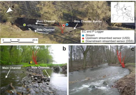
Fig. 2. (a) Aerial photograph (source: K¨unzelmann, UFZ) of the

studied in-stream gravel bar showing the location of the EC and pressure sensors, (b) the gravel bar during low flow (note the hy-draulic gradient between the main channel and the side channel),

(c) the same spot during high flow with the gravel bar submerged

and the side channel fully connected. During high flow the lateral hydraulic gradients are absent. The tree marked in red is the same in each picture for better orientation.

al. (2006). The hydraulic gradients between the stream and the groundwater have been found to alternate seasonally based on stream water level data and head measurements in adjacent groundwater monitoring wells. The in-stream gravel bar is characterised by visually observable lateral hydraulic gradients between the main and the side channel (Fig. 2b). The differences in water level arise from the steeper slope of the side channel at the upstream end of the gravel bar. As the stream flow increases this morphologic effect levels off (Fig. 2c).

The mean EC is lowest in the stream with 576 µS cm−1. In the stream bed the mean EC is 588 µS cm−1at the USS and 601 µS cm−1at the DSS location, respectively. These values are similar to observed EC values measured manually in ob-servation wells located close to the stream banks indicating the mixing of stream water with the adjacent groundwater. EC of groundwater that is potentially not influenced by the stream is around 1020 to 1170 µS cm−1manually measured in two wells located approximately 160 m and 500 m away from the left and right river banks, respectively.

3.2 Experimental setup and data collection

Screen LTC Logger

Threaded lid

Fig. 3. Conceptual sketch of the pressure tight steel tube for the

logger installations.

at the 2 cm long screen at the bottom of the device (Fig. 3). Unlike with a piezometer, the top of the tube is at level with the stream bed surface and does not rise into the water col-umn to avoid any surface flow obstruction. After the logger deployment, the tube is closed with a threaded lid at the top to ensure that the pressure measurements are not affected by hydrostatic pressure when the device is submerged. The cen-tre of the screen of each tube is located at a depth of 0.44 m below the stream bed surface. The accuracies of the sensors as reported by the manufacturer are 1 cm for pressure, 0.1◦C for temperature and 20 µS cm−1 for EC. Measured EC val-ues are internally compensated for temperature to derive spe-cific electrical conductivities normalised to 25◦C. Through-out the paper we refer to the temperature-compensated EC. The data was recorded at a 10 min interval between 13 July and 2 September 2011.

4 Results

4.1 Time series data

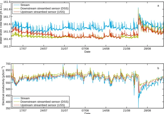
Figure 4a shows the water level in the stream and the total hy-draulic head recorded in the stream bed (m a.s.l.). Generally, during the data collection period in summer 2011 losing con-ditions were prevalent. However, the flood pulse around the 25 August apparently diminishes the hydraulic head differ-ences. Superimposed onto the general water level are short-term pulse-like fluctuations which increase the water level by 5 to 10 cm. These peaks are due to mill operations upstream of the study site.

The general pattern of EC inversely follows the water level of rain events. High water level and thus stream flow is as-sociated with lower EC due to a dilution effect of rain wa-ter (Fig. 4b). The mill-induced, pulse-like wawa-ter level fluc-tuations also decrease the EC but not to the same extent as rain events. Variations of EC in the stream range between 354 and 694 µS cm−1.The lowest value was observed during

the flood event and was interpreted as a dilution effect. The EC variation in the stream has an approximate mean period of 16 h. The mean period was estimated based on the num-ber of zero crossings of the entire EC signal (normalised to zero mean). The mean EC amplitude in the stream during one period is 21 µS cm−1. The EC signal in the stream bed lags the stream signal at both the USS and DSS location. The time lags between the stream and the stream bed sensors change over time. As illustrated in Fig. 5a between 17 July and 19 July, the DSS response occurs later than the one at the USS. Between 18 August and 20 August, for example, the USS response occurs before the DSS response (Fig. 5b). The characteristic features and amplitudes in all time series are similar, indicating no general dampening or smearing of the signal. This indicates short flow paths. However, we have detected a period with low correlation between the stream and the stream bed EC around 24 and 25 July (Figs. 5c, 6). The short-term fluctuations (double peak) of EC do not prop-agate sufficiently deep into the sediment to be detected by the stream bed sensors (Fig. 5c). The damping of the varying EC signal depends not only on dispersion and diffusion but also on the frequency.

4.2 Time lags

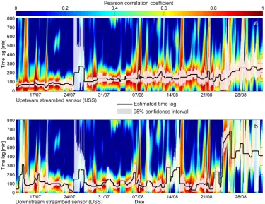
Figure 6 shows the estimates of the characteristic transient time lags for the USS and DSS and the underlying correla-tion matrix d(ai, bj)r rotated by 45◦to map the diagonal on

the x-axis. The mean time lags of both stream bed sensors are similar with 2 h 21 min for the USS and 2 h 54 min for the DSS, respectively. However, the DSS is characterised by a shorter mode of 1 h 40 min, while the mode of the USS is 2 h 20 min. At the downstream location a wider range of time lags was observed than at the USS location (standard devia-tions: USS 56 min, DSS 2 h 29 min). For comparison cross-correlation analysis reveals a time lag of 2 h for the USS and 1 h 40 min for the DSS. These values are exactly (1 h 40 min) and close to (2 h 20 min), respectively, the modes of the tran-sient time lag.

During and after the flood event between 24 and 25 Au-gust occur the highest differences of the estimated time lags. Clearly the USS shows a different response to the flood event. The time lag remains relatively unaffected. This is in accor-dance with the hydraulic gradient. At the peak of the flood event the hydraulic head difference almost reached zero at the DSS location, while at the USS a smaller but still losing gradient was observed. Accordingly, at the DSS location the time lag quickly increases during the flood pulse from less than 2 h to 11 h and remains high for the rest of the analysed time span. Thus, the USS and DSS locations have a different response to flood pulse for both the hydraulic gradient and the EC – based characteristic time lag.

a

Date

Water level/ Total head [m a.s.l.]

17/07 24/07 31/07 07/08 14/08 21/08 28/08

161.3 161.4 161.5 161.6 161.7 161.8 161.9

Stream

Downstream streambed sensor (DSS) Upstream streambed sensor (USS)

17/07 24/07 31/07 07/08 14/08 21/08 28/08

350 400 450 500 550 600 650 700

b

Date

Electrical conductivity [µScm

−1

]

Stream

Downstream streambed sensor (DSS) Upstream streambed sensor (USS)

Fig. 4. (a) Time series of water level in the Selke River (blue) and hydraulic heads in the stream bed at the USS and DSS location of the

gravel bar. (b) Time series of electrical conductivity.

Double peak

Fig. 5. Close-up of EC fluctuations for three two-day windows (a) the DSS lags behind the USS (b) USS lags behind the DSS (c) a period

with low correlation coefficients. The double peak in the stream EC signal does not propagate to the stream bed sensors.

from downwelling of stream water at the upstream side of the gravel bar (at the USS) and reemergence at the downstream end (at the DSS) would have caused an observable dampen-ing of the signal and a longer time shift at the DSS.

The correlation matrices optically reveal the band of high correlation that encloses the optimal MCP (Fig. 6a and b). In general, there is an excellent correlation of the EC time se-ries along the (MCP), whose correlations coefficients (rMCP) have a mean of 0.80 at the downstream and 0.87 at the USS. Median values of 0.84 and 0.91 indicate that the distribution is slightly skewed towards higherrMCP.

For both sensors vertical bands of high correlation occur. These high correlation bands have a similar timing and shape for both sensors. They are a result of low amplitudes in the stream EC signal. An extreme case would be a constant sig-nal with no variations. This would result in a correlation

Fig. 6. Correlation matrices of the DSS and USS. Solid black line: characteristic transient time lag at the (a) USS (b) DSS location. Shaded

white area: 95 % confidence interval. The data is truncated to visualise only the range of the time lags.

5 Discussion and conclusion

The time-varying lag of the EC signal between the stream and the stream bed sensor can be interpreted as the advec-tive travel time of water. Knowing the lengths of the flow paths would provide flow velocities. However, the true flow paths remain unknown. The vertical component of the total flow vector in the stream bed can be estimated from the time lag and the depths of the sensors. The distance between the stream bed surface and the sensor location is the shortest pos-sible flow path. At the USS and DSS, the mean apparent ver-tical flow velocities are 5.4 m d−1with a standard deviation of 2.6 m d−1 and 6.3 m d−1(standard deviation: 5.3 m d−1), respectively. The velocities from the shortest possible flow path represent the lower bound since longer flow paths would require higher velocities for the same time lag. The flow ve-locities are similar to that estimated based on Darcy’s law from hydraulic head measurements. Vertical hydraulic gra-dients may not provide a good indication for direction and magnitude of water flow particularly under variable hydro-logic conditions (K¨aser et al., 2009). Apart from the good match during the flood event, hydraulic head differences and EC time lag are not always consistent. Some uncertainty arises from the stream water level data during very low flows where the depth of the water column is close to the limit of the applicability of the pressure sensor. However, there are

other observations that cannot be attributed to measurement errors. For instance there is no indication in the hydraulic data for the relatively high time lag at the downstream sensor at the beginning of the observation period. Moreover, the ex-tremely short time lag on 24 August can also not be explained from the hydraulic head difference at this time.

The original DTW-approach is prone to noisy estimates of travel times. The DTW algorithm may also produce singular-ities where several points in time in one series are mapped to a single point in the other time series. To avoid noise and sin-gularities the standard DTW algorithm was modified by ap-plying a sliding window to ensure smooth and unique travel time variations. The method generally provides robust results when no pronounced damping of the output signal by diffu-sion and disperdiffu-sion occurs. The characteristic shape of the input and output signal should be nearly the same as it is in our case. However, similarly to cross-correlation analysis a filter can be applied to the input series in order to obtain a similar degree of smoothness for both time series.

coefficients over a range of possible time lags are caused by small gradual EC variations or portions of the EC time series that contain little or no fluctuations on the time scale of the sliding window length.

By using the correlation coefficient as distance measure in the proposed sliding window DTW, the resulting distance matrix is basically the same as for windowed cross correla-tion providing the windows are shifted by a single time step. However, both methods start from different points. Cross cor-relation is typically applied for the entire data series, whereas windowing allows to estimate the cross-correlation function for subsequences of the data. DTW was originally developed for element wise alignment of series. Aligning subsequences of the data series can be viewed as a kind of upscaling from the element perspective, while windowed cross correlation represents a downscaling from the entire-series perspective. Despite this similarity DTW has particular advantages com-pared to cross correlation with sliding window. First, the dis-tance measure is not limited to the correlation coefficient and can be selected based upon the individual problem, i.e. the conventional measure is Euclidean distance. Second, in cross correlation with sliding window the window size and the maximum lag depend on each other. Searching for larger lags requires larger windows. In DTW analysis they are in-dependent since the optimal distance is found by searching the entire distance matrix rather than only the subsequences in the window.

In DTW the time series are optimally aligned by finding the minimum cost path through the distance matrix. Thus, the transient time shift that is required to optimally align to time series is also inherent in the minimum cost path. As such this provides an automated method to detect the time lags between two signals. A similar algorithm could be used to automatically extract the optimal alignment from a win-dowed cross-correlation matrix.

The transient DTW based time series analysis can provide insights into the temporal dynamics of advective travel times in the stream beds that are not easily obtained from other methods. Using a sliding window instead of element by ele-ment warping makes the methods less sensitive to noise.

Acknowledgements. The research was supported by TERENO (Terrestrial Environmental Observatories) and by a grant from the Ministry of Science, Research and Arts of Baden-W¨urttemberg (AZ Zu 33-721.3-2) and the Helmholtz Centre for Environmental Research, Leipzig (UFZ). We would like to thank the anonymus reviewers for their constructive comments.

The service charges for this open access publication have been covered by a Research Centre of the Helmholtz Association.

Edited by: P. Grathwohl

References

Bianchin, M., Smith, L., and Beckie, R.: Quantifying hyporheic ex-change in a tidal river using temperature time series, Water Re-sour. Res., 46, W07507, doi:10.1029/2009WR008365, 2010. Boano, F., Demaria, A., Revelli, R., and Ridolfi, L.:

Biogeochemi-cal zonation due to intrameander hyporheic flow, Water Resour. Res., 46, W02511, doi:10.1029/2008WR007583, 2010. Boker, S., Xu, M., Rotondo, J., and King, K.: Windowed

cross-correlation and peak picking for the analysis of variability in the association between behavioral time series, Psychol. Methods, 7, 338–355, doi:10.1037//1082-989X.7.3.338, 2002.

Briggs, M. A., Lautz, L. K., McKenzie, J. M., Gordon, R. P., and Hare, D. K.: Using high-resolution distributed tem-perature sensing to quantify spatial and temporal variability in vertical hyporheic flux, Water Resour. Res., 48, W02527, doi:10.1029/2011WR011227, 2012.

Calles, U. M.: Diurnal variations in electrical conductivity of water in a small stream, Nord. Hydrol., 13, 157–164, 1982.

Cirpka, O. A., Fienen, M. N., Hofer, M., Hoehn, E., Tessarini, A., Kipfer, R., and Kitanidis, P. K.: Analyzing bank filtration by de-convoluting time series of electric conductivity, Ground Water, 45, 318–328, doi:10.1111/j.1745-6584.2006.00293.x, 2007. Conant, B.: Delineating and quantifying ground water discharge

zones using streambed temperatures, Ground Water, 42, 243– 257, 2004.

Constantz, J.: Heat as a tracer to determine streambed water exchanges, Water Resour. Res., 44, W00D10, doi:10.1029/2008WR006996, 2008.

Findlay, S: Importance of Surface-Subsurface Exchange in Stream Ecosystems – the Hyporheic Zone, Limonol. Oceanogr., 40, 159–164, 1995.

Geist, J. and Auerswald, K.: Physicochemical stream bed character-istics and recruitment of the freshwater pearl mussel, Freshwater Biol., 52, 2299–2316, 2007.

Hatch, C. E., Fisher, A. T., Revenaugh, J. S., Constantz, J., and Ruehl, C.: Quantifying surface water-groundwater in-teractions using time series analysis of streambed thermal records: Method development, Water Resour. Res., 42, W10410, doi:10.1029/2005WR004787, 2006.

Kasahara, T. and Wondzell, S. M.: Geomorphic controls on hy-porheic exchange flow in mountain streams, Water Resour. Res., 39, 1005–1019, doi:10.1029/2002WR001386, 2003.

K¨aser, D. H., Binley, A., Heathwaite, A. L., and Krause, S.: Spatio-temporal variations of hyporheic flow in a riffle-step-pool se-quence, Hydrol. Process., 23, 2138–2149, doi:10.1002/hyp.7317, 2009.

Keery, J., Binley, A., Crook, N., and Smith, J. W.: Temporal and spatial variability of groundwater-surface water fluxes: Develop-ment and application of an analytical method using temperature time series, J. Hydrol., 336, 1–16, 2007.

Keogh, E. J. and Pazzani, M. J.: Derivative dynamic time warp-ing, in: First SIAM International Conference on Data Minwarp-ing, Chicago, IL, 2001.

Ort, C. and Siegrist, H.: Assessing wastewater dilution in small rivers with high resolution conductivity probes, Water Sci. Tech-nol., 59, 1593, doi:10.2166/wst.2009.174, 2009.

Rau, G. C., Andersen, M. S., and Acworth, R. I.: Experimen-tal investigation of the thermal time series method for sur-face water-groundwater interactions, Water Resour. Res., 48, W03530, doi:10.1029/2011WR011560, 2012

Sakoe, H. and Chiba, S.: Dynamic-Programming Algorithm Opti-mization for Spoken Word Recognition, IEEE T. Acoust. Speech, 26, 43–49, doi:10.1109/TASSP.1978.1163055, 1978.

Salehin, M., Packman, A., and Zaramella, M.: Hyporheic exchange with gravel beds: Basic hydrodynamic interactions and bedform-induced advective flows, J. Hydraul. Eng.-ASCE, 130, 647–656, 2004.

Sawyer, A. H. and Cardenas, M. B.: Hyporheic flow and residence time distributions in heterogeneous cross-bedded sediment, Wa-ter Resour. Res., 45, W08406, doi:10.1029/2008WR007632, 2009.

Sawyer, A., Cardenas, M., Bomar, A., and Mackey, M.: Impact of dam operations on hyporheic exchange in the riparian zone of a regulated river, Hydrol. Process., 23, 2129–2137, 2009. Schmidt, C., Bayer-Raich, M., and Schirmer, M.:

Characteriza-tion of spatial heterogeneity of groundwater-stream water in-teractions using multiple depth streambed temperature measure-ments at the reach scale, Hydrol. Earth Syst. Sci., 10, 849–859, doi:10.5194/hess-10-849-2006, 2006.

Schmidt, C., Conant, B., Bayer-Raich, M., and Schirmer, M.: Eval-uation and field-scale application of an ana analytical method to quantify groundwater discharge using mapped streambed tem-peratures, J. Hydrol., 347, 292–307, 2007.

Schmidt, C., Martienssen, M., and Kalbus, E.: Influence of wa-ter flux and redox conditions on chlorobenzene concentrations in a contaminated streambed, Hydrol. Process., 25, 234–245, doi:10.1002/hyp.7839, 2011.

Sheets, R., Darner, R., and Whitteberry, B.: Lag times of bank fil-tration at a well field, Cincinnati, Ohio, USA, J. Hydrol., 266, 162–174, doi:10.1016/S0022-1694(02)00164-6, 2002.

Stonedahl, S. H., Harvey, J. W., W¨orman, A., Salehin, M., and Packman, A. I.: A multiscale model for integrating hyporheic exchange from ripples to meanders, Water Resour. Res., 46, W12539, doi:10.1029/2009WR008865, 2010.

Storey, R. G., Howard, K. W. F., and Williams, D. D.: Fac-tors controlling riffle-scale hyporheic exchange flows and their seasonal changes in a gaining stream: A three-dimensional groundwater flow model, Water Resour. Res., 39, 1034, doi:10.1029/2002WR001367, 2003.

Triska, F. J., Du, J. H., and Avanzino, R. J.: The role of water ex-change between a stream channel and its hyporheic zone in ni-trogen cycling at the terrestrial-aquatic interface, Hydrobiologia, 251, 167–184, 1993.

Valett, H.: Surface-hyporheic interactions in a Sonoran Desert stream – Hydrologic exchange and diel periodicity, Hydrobiolo-gia, 259, 133–144, doi:10.1007/BF00006593, 1993.

Vogt, T., Schneider, P., Hahn-Woernle, L., and Cirpka, O. A.: Es-timation of seepage rates in a losing stream by means of fiber-optic high-resolution vertical temperature profiling, J. Hydrol., 380, 154–164, 2010a.

Vogt, T., Hoehn, E., Schneider, P., Freund, A., Schirmer, M., and Cirpka, O. A.: Fluctuations of electrical conductivity as a natural tracer for bank filtration in a losing stream, Adv. Water Resour., 33, 1296–1308, 2010b.

Westbrook, S., Rayner, J., Davis, G., Clement, T., Bjerg, P., and Fisher, S.: Interaction between shallow groundwater, saline sur-face water and contaminant discharge at a seasonally and tidally forced estuarine boundary, J. Hydrol., 302, 255–269, 2005. Wroblicky, G., Campana, M., Valett, H., and Dahm, C.: Seasonal