A new remote hazard and risk assessment framework for glacial lakes in the Nepal Himalaya

www.hydrol-earth-syst-sci.net/20/3455/2016/ doi:10.5194/hess-20-3455-2016

© Author(s) 2016. CC Attribution 3.0 License.

A new remote hazard and risk assessment framework for glacial

lakes in the Nepal Himalaya

David R. Rounce1, Daene C. McKinney1, Jonathan M. Lala1, Alton C. Byers2, and C. Scott Watson3 1_{Center for Research in Water Resources, University of Texas at Austin, Austin, TX, USA}

2_{Institute of Arctic and Alpine Research, University of Colorado Boulder, Boulder, CO, USA} 3_{School of Geography, University of Leeds, Leeds, LS2 9JT, UK}

Correspondence to:David R. Rounce ([email protected])

Received: 8 April 2016 – Published in Hydrol. Earth Syst. Sci. Discuss.: 13 May 2016 Revised: 31 July 2016 – Accepted: 9 August 2016 – Published: 31 August 2016

Abstract. Glacial lake outburst floods (GLOFs) pose a sig-nificant threat to downstream communities and infrastructure due to their potential to rapidly unleash stored lake water. The most common triggers of these GLOFs are mass movement entering the lake and/or the self-destruction of the terminal moraine due to hydrostatic pressures or a buried ice core. This study initially uses previous qualitative and quantita-tive assessments to understand the hazards associated with eight glacial lakes in the Nepal Himalaya that are widely con-sidered to be highly dangerous. The previous assessments yield conflicting classifications with respect to each glacial lake, which spurred the development of a new holistic, re-producible, and objective approach based solely on remotely sensed data. This remote hazard assessment analyzes mass movement entering the lake, the stability of the moraine, and lake growth in conjunction with a geometric GLOF to de-termine the downstream impacts such that the present and future risk associated with each glacial lake may be quanti-fied. The new approach is developed within a hazard, risk, and management action framework with the aim that this remote assessment may guide future field campaigns, mod-eling efforts, and ultimately risk-mitigation strategies. The remote assessment was found to provide valuable informa-tion regarding the hazards faced by each glacial lake and re-sults were discussed within the context of the current state of knowledge to help guide future efforts.

1 Introduction

self-destructive events as they lump the failure from the degra-dation of buried ice, hydrostatic pressure, and/or the effects of time all together due to the difficulty of distinguishing the exact cause of failure. Similarly, Richardson and Reynolds (2000) were unable to identify the cause of over 23 % of the GLOFs in their study due to a lack of information. This un-certainty regarding other mechanisms of failure stresses the importance of taking a holistic approach towards assessing the hazard of these glacial lakes that accounts for the various triggering mechanisms and the stability of the moraine.

Methods have been developed to characterize the hazard and risk associated with glacial lakes in Cordillera Blanca (Reynolds, 2003; Hegglin and Huggel, 2008; Emmer and Vilímek, 2013, 2014), New Zealand (Allen et al., 2009), North America (Clague and Evans, 2000; O’Connor et al., 2001; McKillop and Clague, 2007a, b), the Swiss Alps (Huggel et al., 2004b; Nussbaumer et al., 2014), the Hi-malaya (Wang et al., 2008, 2012; ICIMOD, 2011; Fujita et al., 2013; Worni et al., 2013), the Tibetan Plateau (Wang et al., 2011), and other parts of high-mountain Asia (Bolch et al., 2011; Mergili and Schneider, 2011). These methods vary considerably based on the parameters considered, the level of importance placed upon each parameter, the amount and type of required input data, their ability to be transferred to other regions, and their levels of objectivity. Emmer and Vilímek (2013) applied a suite of existing hazard assessments to glacial lakes in Cordillera Blanca and found good agree-ment between the various methods despite the various stud-ies using different parameters, various amounts of qualitative and quantitative information, and them being developed for specific regions. This good agreement suggests it may be fea-sible to accurately classify the hazard of a glacial lake and shows the parameters may be qualitative or quantitative as long as the developed analysis and thresholds are objective.

Unfortunately, the use of various approaches can also lead to different classifications of the hazard associated with an in-dividual glacial lake. Imja Tsho (“Tsho” is Tibetan for lake), located in the Everest region of Nepal, provides an excel-lent example of these conflicting classifications. Some stud-ies have stated that Imja Tsho is safe (Watanabe et al., 2009; Fujita et al., 2013), a very low risk (Hambrey et al., 2008), or a moderate risk (Budhathoki et al., 2010). Conversely, ICI-MOD (2011) identified Imja Tsho as one of six glacial lakes in Nepal that is a high priority for further investigation, and currently remediation efforts to reduce its hazard are under-way (UNDP, 2013). These remediation efforts and a similar project completed at Tsho Rolpa (Rana et al., 2000) are ex-cellent steps forward for Nepal with respect to addressing the hazards associated with its glacial lakes. However, it is im-portant that these efforts and resources are properly directed to ensure the development of the most cost-effective, Nepal-specific methods for successfully reducing the risk of glacial lakes as practiced by the Peruvians since the 1950s (Carey, 2010). Conflicting classifications of Imja Tsho suggest re-lief efforts may be misguided if the lake is indeed safe and

also send mixed signals to the general public and downstream communities that these studies are meant to assist. Another good example of these conflicting reports is Chamlang South Tsho (also referred to as West Chamlang), where one study stated the lake was not particularly dangerous (Byers et al., 2013) and another stated the lake was potentially dangerous (Lamsal et al., 2016), despite having access to the same data sets.

These various assessments and conclusions highlight the importance of (1) developing a clear and straightforward holistic method for assessing the hazard associated with a glacial lake and (2) constructing a framework that guides management actions for a given glacial lake that accounts for the various levels of data collection, modeling, and field campaigns. An additional aspect that is important to incorpo-rate is how the hazard associated with these glacial lakes will change as the glacier and glacial lakes continue to evolve. The negative mass balance regime across the central Hi-malaya (Kääb et al., 2012) will affect the continued growth of existing lakes and development of new lakes in overdeep-ened basins (Linsbauer et al., 2016). Anticipating this future development is especially important when one considers that successful remediation strategies on hazardous lakes often take more than a decade to secure funding and implement (Quincey et al., 2007).

This study assesses the performance of existing hazard as-sessment methods on potentially dangerous glacial lakes in Nepal to determine how well they agree with one another. These existing studies are used as the basis for developing a new holistic approach that is objective, repeatable, and uses readily available information such that it may be applied to any glacial lake. This approach will be developed within a management action framework such that it may be used to guide future field campaigns, research, and ultimately risk-mitigation strategies associated with hazardous glacial lakes.

2 Study area

This study assesses the hazard and risk of GLOFs for eight proglacial lakes in the Nepal Himalaya (Fig. 1). Six of these glacial lakes were identified by ICIMOD (2011) as being high priority for further investigation: Tsho Rolpa, Lower Barun Tsho, Imja Tsho, Lumding Tsho (also referred to as Tsho Og), Chamlang South Tsho (also referred to as West Chamlang), and Thulagi Tsho. The other two glacial lakes considered are Chamlang North Tsho (also referred to as Lake 464), which was found to be dangerous (Byers et al., 2013), and Dig Tsho, which experienced a GLOF in 1985 (Vuichard and Zimmermann, 1987). The level of investiga-tion of each of lake is highly variable.

ICI-MOD (2011) provides a detailed review of the development of these lakes and the field investigations that have been performed to measure the bathymetry, use geophysical tech-niques to identify the presence of buried ice, and broadly in-vestigate the hazard associated with these lakes. Since this study, the stability of their terminal moraines has been inves-tigated (Fujita et al., 2013) and potential GLOFs have been modeled (Khanal et al., 2015). Additionally, a laboratory ex-periment was conducted to model the stability of Tsho Rolpa (Shrestha et al., 2012) and other detailed investigations of Imja Tsho’s bathymetry (Somos-Valenzuela et al., 2014) and potential floods (Bajracharya et al., 2007; Somos-Valenzuela et al., 2015) have been conducted. Tsho Rolpa is also the only glacial lake in Nepal that has been remediated in an effort to reduce its hazard and subsequently was extensively studied in the field prior to its remediation (Richardson and Reynolds, 2000), while remediation efforts are currently under way for Imja Tsho (UNDP, 2013).

Dig Tsho (86◦35.10E, 27◦52.50N, 4365.9 m a.s.l.) has been extensively studied and used as a site to assess and improve GLOF models (Cenderelli and Wohl, 2001; Ba-jracharya et al., 2007; Westoby et al., 2014, 2015; Watson et al., 2015). Chamlang South Tsho (86◦57.50E, 27◦45.30N, 4951.8 m a.s.l.) and Chamlang North Tsho (86◦57.30E, 27◦47.00N, 5218.0 m a.s.l.) were both investigated in the field by Byers et al. (2013), which also included the mod-eling of a GLOF from Chamlang North Tsho. Chamlang South Tsho has since been further investigated using high-resolution digital elevation models (DEMs) and a bathy-metric survey (Sawagaki et al, 2012; Lamsal et al., 2016). A field investigation was performed at Lower Barun Tsho (87◦_05.70_{E, 27}◦_47.90_{N, 4534.5 m a.s.l.) in 1993 in}

connec-tion with potential hydropower systems downstream (Mool et al., 2001), but has received little attention since with the exception of a visual field assessment of the terminal moraine and potential triggers (Byers et al., 2014). Similarly, Lumding Tsho (86◦36.80E, 27◦46.80N, 4819.3 m a.s.l.) has received little attention beyond documenting its growth (Ba-jracharya and Mool, 2009) despite being identified as a high priority glacial lake (ICIMOD, 2011). This study addresses this data gap and shows how a new method and framework may be used to prioritize future glacial lake investigations and management actions.

3 Existing methods 3.1 Summary

The first method that was used to assess the hazard of these eight glacial lakes was a “shotgun approach” to determine how their classifications vary using previous qualitative and quantitative assessment methods. The shotgun approach uses the same studies as Emmer and Vilímek (2013) with the ex-ception of Clague and Evans (2000) and Grabs and Hanisch

Figure 1.The locations of the eight glacial lakes assessed in this study in the Nepal Himalaya.

(1993) as these required site-specific knowledge that was not possible to obtain from remote sensing. The use of solely remotely sensed data is one of the main goals of the new method and framework developed in this study. The qualita-tive methods used were O’Connor et al. (2001), Costa and Schuster (1988), and Wang et al. (2008). Wang et al. (2008) highlights 10 hazard parameters, but only gives thresholds for 8 of them; therefore, the 8 parameters with thresholds are used for this qualitative approach. As a specific hazard rating is unable to be determined from these qualitative approaches, the arithmetic mean of the three is used to rank the glacial lakes.

overtop-Table 1.Previous qualitative hazard assessments applied to eight glacial lakes in Nepal. Fractions are the number of hazard parameters identified out of the total number of parameters used by each method. Details shown in Tables S.1–S.3.

Lake O’Connor et al. (2001) Costa and Schuster (1988) Wang et al. (2008) Arithmetic mean

Chamlang North Tsho 2/2 3/4 6/8 0.83

Chamlang South Tsho 2/2 3/4 6/8 0.83

Dig Tsho 2/2 2/4 5/8 0.71

Imja Tsho 1/2 2/4 5/8 0.54

Lower Barun Tsho 2/2 3/4 5/8 0.79

Lumding Tsho 2/2 2/4 6/8 0.75

Thulagi Tsho 1/2 2/4 5/8 0.54

Tsho Rolpa 2/2 3/4 6/8 0.83

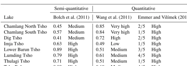
Table 2.Previous semi-quantitative and quantitative hazard assessments applied to eight glacial lakes in Nepal. Values and thresholds for classifications are specific to each study. Fractions are the number of scenarios for each lake that are considered to be highly dangerous. Details shown in Tables S.4–S.6.

Semi-quantitative Quantitative

Lake Bolch et al. (2011) Wang et al. (2011) Emmer and Vilímek (2014)

Chamlang North Tsho 0.45 Medium 0.85 Very high 2/5 High Chamlang South Tsho 0.57 Medium 0.84 Very high 1/5 High

Dig Tsho 0.41 Medium 0.72 High 2/5 High

Imja Tsho 0.63 High 0.49 Low 1/5 High

Lower Barun Tsho 0.89 High 0.51 Medium 3/5 High

Lumding Tsho 0.79 High 0.61 Medium 4/5 High

Thulagi Tsho 0.71 High 0.51 Medium 1/5 High

Tsho Rolpa 0.89 High 0.60 Medium 4/5 High

ping from a flood upstream, (3) moraine failure due to mass movement entering the lake, (4) moraine failure from a flood upstream, and (5) failure resulting from a strong earthquake. Unfortunately, the locations of seepage points required for the last scenario were not identifiable from remote sensing, so the dam instability due to piping was not accounted for. 3.2 Application of existing methods

The qualitative hazard assessments show a good deal of vari-ation between the three approaches (Table 1). The arithmetic mean reveals the most dangerous lakes based on these three qualitative approaches are Chamlang North Tsho, Chamlang South Tsho, and Tsho Rolpa, closely followed by the oth-ers with the exception of Imja Tsho and Thulagi Tsho. Imja Tsho has a lower value since these methods all use some form of mass movement entering the lake, which currently is not a threat at Imja Tsho. Thulagi Tsho is also not sus-ceptible to ice avalanches and by some methods has a more stable moraine due to the presence of vegetation. The semi-quantitative and semi-quantitative assessments give very different classifications of the hazard associated with each lake (Ta-ble 2). Bolch et al. (2011) emphasize the size of the lake and its ability to expand, so all the large glacial lakes that have expanded over the last decade are ranked as high dan-ger (Imja Tsho, Lower Barun Tsho, Lumding Tsho,

Thu-lagi Tsho, and Tsho Rolpa). The other glacial lakes that have already reached their maximum extent are classified as medium danger. Wang et al. (2011) is the complete oppo-site since the glacial lakes that have already reached their maximum extent are all high risk or very high risk, while the others are medium or low risk. This conflicting classifi-cation is due to the emphasis on parameters associated with mass movement entering the lake, i.e., both the distance and the slope between the lake and the glacier. The large glacial lakes that are still expanding have gentle slopes behind their calving fronts, which cause them to be classified as medium or low.

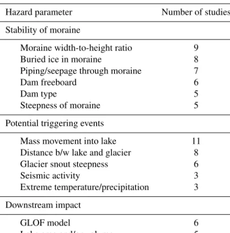
Table 3.Most frequently used parameters associated with previous studies (adapted from Emmer and Vilímek, 2013).

Hazard parameter Number of studies

Stability of moraine

Moraine width-to-height ratio 9

Buried ice in moraine 8

Piping/seepage through moraine 7

Dam freeboard 6

Dam type 5

Steepness of moraine 5

Potential triggering events

Mass movement into lake 11

Distance b/w lake and glacier 8

Glacier snout steepness 6

Seismic activity 3

Extreme temperature/precipitation 3

Downstream impact

GLOF model 6

Lake area and/or volume 5

developed for scenarios related to Cordillera Blanca such that the framework could be transferred to other regions, but the exact scenarios or parameters used may not be representa-tive of the main threats to other regions. Nonetheless, the assessment yields valuable insight showing Lumding Tsho, Lower Barun Tsho, and Tsho Rolpa have the greatest num-ber of hazard scenarios due to the potential for a flood from a glacial lake upstream, which is important to consider.

The shotgun approach shows that the hazard classification of each glacial lake varies greatly depending upon the se-lected method, which makes classifying the hazard associ-ated with a particular glacial lake difficult. Fortunately, the shotgun approach is useful as it highlights the most com-monly used parameters in previous studies. Table 3 shows the most frequently used parameters are mass movement enter-ing the lake, the moraine width-to-height ratio, the presence of buried ice in the moraine, and the distance between the lake and the glacier. These naturally reflect the most common causes of GLOFs, i.e., mass movement entering the lake and the self-destruction of the moraine due to hydrostatic pres-sure and/or the degradation of buried ice (Richardson and Reynolds, 2000; Wang et al., 2012; Emmer and Cochachin, 2013). Furthermore, many of the other parameters are sim-ply alternative forms of estimating the potential cause of fail-ure; e.g., glacier snout steepness or the distance between the lake and the glacier are surrogate ways to estimate whether the lake is susceptible to an avalanche entering the lake. In this manner, the shotgun approach lends insight into the var-ious parameters or methods that were used to estimate dif-ferent triggering events. The variety of parameters and the frequency of their use highlight the parameters that are

im-Figure 2.Schematic of GLOF hazard parameters used in the new method: (1) snow/ice avalanche, (2) rockfall, (3) flood from up-stream lake, (4) lake expansion, (5) hydrostatic pressure, (6) ice-cored moraine, and (7) downstream impact.

portant to consider in addition to highlighting the importance of developing a holistic method that accounts for these vari-ous forms of failure.

4 New hazard and risk framework

be detailed in the discussion in conjunction with a brief de-scription of the current state of knowledge for each glacial lake investigated.

4.1 Remote hazard assessment: methods

The remote hazard assessment framework is intended to be used as a launching point for assessing the hazards of glacial lakes. The parameters and models used in this framework are all derived from globally available data sets. The DEM uti-lized in this study is the ASTER GDEM, which is composed of automatically generated DEMs from the Advanced Space-borne Emission and Reflection radiometer (ASTER) stereo scenes acquired from 2000 to 2008. The ASTER GDEM V2 (hereon referred to as GDEM) has a horizontal resolution of 30 m and a vertical RMSE of±15.1 m for mountainous areas (ASTER GDEM Validation Team, 2011). The GDEM was used in this study instead of the SRTM V4 DEM (Farr et al., 2007) due to its higher resolution, and its effect on the flood models is discussed in Sect. 4.1.4. Landsat imagery (Land-sat 4/5 TM, Land(Land-sat 7 ETM+, and Landsat 8 OLI TIRS) was also used to delineate the glacial lakes and identify areas of snow/ice and land. Landsat imagery was selected for this study as it is the highest-resolution multi-spectral imagery that is ubiquitous.

4.1.1 Mass movement trajectories

Mass movement entering a glacial lake is a highly haz-ardous situation for glacial lakes as the entry may cause a tsunami-like displacement wave that can trigger a GLOF. This study considers three types of dynamic failures: snow/ice avalanches, rockfalls/landslides, and upstream GLOFs (Fig. 2). This section describes the mass move-ment trajectories for avalanches and rockfalls, while the up-stream GLOFs are discussed later (Sect. 4.1.5). Landsat im-agery was used to automatically detect glacierized and non-glacierized areas using a ratio of the NIR and SWIR 1 bands with a threshold of 2.2 (Huggel et al., 2004a). In this sim-plified model, there is no differentiation between snow and ice. Snow/ice avalanche-prone areas were identified as any glacierized area with a slope greater than 45◦(Alean, 1985) but less than 60◦, as mass is unlikely to accumulate beyond this threshold (Osti et al., 2011; Shea et al., 2015). Rockfall-prone areas were identified as any non-glacierized areas with a slope greater than 30◦ (Bolch et al., 2011). In this case, the term rockfall is meant to refer to any mass movement from a non-glacierized area and hence is meant to include landslides as well. The lateral moraines were precluded from being rockfall-prone areas as they tend to be fairly well de-veloped and are unlikely to lose a large amount of material in a single event. A single flow model using the flow direc-tion algorithm in ArcGIS 10.3 in conjuncdirec-tion with a sink-free GDEM was used to model the path of the mass movement.

The runout distance of the mass movement trajectories was computed using an average slope threshold of 17 and 20◦ _{for avalanches and rockfalls, respectively. However,}

avalanches with a volume less than 6.67 million cubic meters had a higher average slope threshold based on a log relation-ship between avalanche volume and average trajectory slope (Huggel et al., 2004b):

tan(α)=1.111−0.118 log(V ). (1)

The avalanche volume was determined from estimates of avalanche-prone areas and assumed avalanche thickness. Avalanche-prone area was estimated using a variable ker-nel filter with a 90 % threshold to determine the maximum avalanche-prone area with each pixel. The variable kernel fil-ter begins with an individual pixel and defil-termines whether 90 % of the surrounding pixels including itself, i.e., a 3×3 pixel grid, are avalanche-prone. If this condition is satis-fied, then the kernel filter increases by one pixel, i.e., a 5×5 pixel grid, and continues this process until the 90 % threshold fails. The estimated avalanche-prone area is con-sidered to be the largest area that satisfies the 90 % thresh-old. This study assumed three depths for avalanche thickness (10, 30, and 50 m) based on avalanches previously reported in Russia (Huggel et al., 2005) and common estimates in the Swiss Alps (Huggel et al., 2004b) due to a lack of avalanche depth data in the Himalaya. These assumed thicknesses also agree well with ice thickness estimates derived from a re-lationship between thickness, shear stress, slope factor, and slope (Wang et al., 2012). The ice thickness estimates of the avalanche-prone areas based on Wang et al. (2012) ranged from 15 to 48 m, which lends confidence to the assumed range of values (10–50 m) used in this study. These three scenarios were used in conjunction with the avalanche-prone areas to estimate avalanche volume. The avalanche volumes ranged from 2.7×104to 6.7×106m3.

4.1.2 Lake expansion

One difficulty associated with the NDWI analysis is the objective selection of the threshold used to differentiate land and water. Bolch et al. (2011) found the threshold for Land-sat images to range from 0.3 to 0.9 for glacial lakes in north-ern Tien Shan, but no clear instructions exist for selecting the threshold for each image and glacial lake. Thakuri et al. (2015) used the same technique at Imja Tsho and found the lake area to be constant between July and January each year. They suggested this was due to the lake level being con-stant, but measurements of lake level were not included. This study uses the same approach with Landsat imagery from 2000 to 2015 captured between September and January each year and assumes the width of the lake between the lateral moraines is constant based on the findings from Thakuri et al. (2015) and the assumption of a constant lake level. Two exceptions were made, one for Chamlang North Tsho, which used an image from May as there were fewer shadows during this time of year, and another for the supplementary image of Lower Barun Tsho in 2008, which used an image from the following April. Additionally, no clear-sky, non-banded Landsat imagery was available in 2003, 2004, and 2008 for Lower Barun Tsho, so Advanced Spaceborne Thermal Emis-sion and Reflection Radiometer (ASTER) images between September and January were used for these years instead.

Thresholds were objectively selected such that the aver-age width of the lake was constant between imaver-ages. This method forces any changes in lake area to be the result of upglacier and/or downglacier expansion, which is the focus of this study. In the event that clouds or the Landsat 7 strip-ping caused portions of the lake to have gaps in the imagery, a second Landsat image was used to fill in these missing areas using the same criteria. Additionally, large debris-covered icebergs nearing the calving front that could cause pixels to be misclassified as land instead of water were manually cor-rected in post-processing. The maximum error in the lake area estimates was calculated as the perimeter of the lake multiplied by half the pixel resolution (±15 m for Landsat images).

The expansion rate was estimated as the average rate of areal expansion for all the 10-year intervals available; i.e., if yearly delineations were available from 2000 to 2015, then the six values of the 10-year expansion were averaged to es-timate the areal expansion rate. These expansion rates were used in conjunction with ice thickness estimates to determine future lake extents. The ice thickness data used in this study are from the GlabTop2 model (Frey et al., 2014), which es-timates the ice thickness from a DEM and glacier outlines. The ice thickness of the glaciers in this study was upwards of 250 m thick behind the calving front of some lakes. The bed topography of the glaciers was computed as the ice thick-ness subtracted from the surface elevation, which was used to identify potential overdeepenings, i.e., locations in the bed topography that are sinks and allow the lake to expand.

Future lake projections were estimated using the average decadal areal expansion rates over the next 50 years such that

the lake’s risk of future dynamic failures could be assessed. Glacier flowlines were used to guide the direction of the ex-pansion. The lake level was assumed to be constant over the next 50 years and was estimated as the average elevation of all the lake pixels based on the lake extent from 2000, as this elevation should be relatively constant over the time period when DEMs for the GDEM were being captured.

4.1.3 Hydrostatic pressure

The exact cause of failure associated with a moraine that spontaneously fails without any external influence is difficult to pinpoint, but is commonly referred to as “self-destruction” (Yamada, 1998; Emmer and Cochachin, 2013). One cause of self-destruction is when the hydrostatic pressure, the pres-sure a column of water exerts on the moraine, exceeds the structural capacity of the moraine. Many studies account for the moraine stability using a ratio of the moraine width-to-height (Table 2), which is subject to large errors if a global DEM is used (Fujita et al., 2008). Fujita et al. (2013) devel-oped a surrogate parameter known as the steep lakefront area (SLA) using remotely sensed data that is not as susceptible to the uncertainty associated with global DEMs. The SLA is the average slope between the lake and any point within 1000 m of the moraine, which is similar in concept to the mean slope of the moraine based on a 100 m buffer that was used by Wang et al. (2011). The slope of any point within 1000 m of the moraine is meant to capture the steepest slope between the lake and the base of the terminal moraine. Fujita et al. (2013) examined moraines that had previously failed and determined that lakes with a SLA less than 10◦were not susceptible to fail.

This study uses the SLA with a threshold of 10◦_to

deter-mine whether the hydrostatic pressure may cause the moraine to self-destruct. NDWI delineations of the lake area are used to identify the pixels for the SLA calculation. The elevation of these lake pixels was set equal to the average elevation of the glacial lake from the GDEM based on the year 2000 delineation. Furthermore, the SLA was only computed for the main body of the lake; i.e., the SLA was not computed from melt ponds on the damming moraines of the lakes. Ini-tial results of the SLA reported very high values of the SLA due to the elevation changes between adjacent pixels in the GDEM. These values are not representative of the slope of the moraine or the hydrostatic pressure on the moraine, so a 100 m buffer around the lake was used such that the SLA would be accurately captured.

4.1.4 Buried ice

pressure, piping/seepage, and reducing the height of the free-board associated with the terminal moraine (Emmer and Cochachin, 2013). The importance of accounting for ice-cored moraines is apparent from previous studies (Table 2), but requires detailed information regarding the terminal moraine that is typically not available from remotely sensed data. Bolch et al. (2011) used permafrost as a surrogate pa-rameter to suggest the potential of an ice-cored moraine. A similar approach was assessed in this study using permafrost maps (Gruber, 2012); however, a comparison between lakes with known ice cores and the permafrost maps revealed no correlation. McKillop and Clague (2007a) assessed the pres-ence of an ice core according to the shape of the moraine us-ing aerial imagery by assumus-ing that a moraine with a rounded surface with arcuate ridges had an ice core, that a dispropor-tionately large terminal moraine in front of a glacier was po-tentially ice-cored, and a narrow, sharp-crested moraine with an angular cross section was ice-free. Unfortunately, this ap-proach is highly subjective and appears to fail for glacial lakes with ice cores in Nepal. For example, Tsho Rolpa has a narrow terminal and lateral moraine that would suggest its moraine is ice-free; however, it is known to have an ice core (Yamada, 1998; Richardson and Reynolds, 2000; ICIMOD, 2011).

In the field a common approach to determine whether a moraine is ice-cored is by observing ice cliffs or karst topog-raphy (Yamada, 1998; Richardson and Reynolds, 2000; ICI-MOD, 2011). Another common way is to witness changes in the outlet channel over time, which has been observed at Imja Tsho (Watanabe, 1994), Tsho Rolpa (Yamada, 1998), and Thulagi Tsho (ICIMOD, 2011). This study takes a similar ap-proach using satellite imagery and Google Earth to identify the presence of any water on the moraine or any changes in the outlet. If water is present on the moraine or any changes in the outlet are observed, the moraine is assumed to have an ice core. During the analysis, a combination of Google Earth and satellite imagery was found to help differentiate between shadows and water, but it is recommended to err on the side of caution when one is unsure. Unfortunately, the lack of clear thresholds for identifying water on the moraine or changes in the outlet adds a small amount of subjective-ness to this study. However, as this was the most effective and least subjective approach to identifying the presence of buried ice in the moraine, it was used for the remote assess-ment.

4.1.5 GLOF modeling

Flood models play a crucial role in a glacial lake hazard as-sessment as they identify areas at risk, which allows one to determine the downstream impact. Westoby et al. (2014) pro-vides a thorough overview of the various types of floods and types of models that may be used to reconstruct a GLOF. In short, if the flood entrains enough sediment from the moraine and channel downstream, the flood may transform

into a debris flow, which increases the momentum of the flood, thereby increasing the GLOF’s extent and potential damage. The models used to reconstruct these debris flows or GLOFs range from simple computationally inexpensive GIS-based methods to computationally expensive, physically based numerical models. The GIS-based methods typically rely solely on the geometry of the downstream channel from a DEM. Numerical models have been used to resolve the flow of a GLOF in one or two dimensions. The benefit of two-dimensional models is their ability to capture more complex features and flow characteristics, e.g., multi-directional flows or super-elevation of flow around a channel bed (Westoby et al., 2014). The selection of a particular model or method typically depends on data availability and the desired model complexity.

This study explored the use of two computationally inex-pensive flood models: the Modified Single Flow direction (MSF) model developed by Huggel et al. (2003) and the Monte Carlo Least Cost Path (MC-LCP) model developed by Watson et al. (2015). The MSF model is a standard flow direction model that “allows the flow to divert from the steep-est descent direction up to 45◦on both sides” (Huggel et al., 2003). The model requires a sink-filled DEM, a starting point in the form of a polygon, and a set threshold to stop the model based on the average angle between the starting point and the downstream flood. Depending on the selected threshold, the model can be used to estimate debris flows or flash floods. The MC-LCP model uses a Monte Carlo simulation to vary the DEM as a function of its uncertainty while identifying the potential flow path for each simulation using a least cost analysis. This model only simulates the flood extent and does not differentiate between debris flows or flash floods.

Table 4.Descriptions of downstream impact classifications.

Classification Description of downstream impact

Very high Potential loss of life with no warning (lodges/buildings)andthe loss of costly infrastructure (e.g., hydropower)

High Potential loss of life with no warning (lodges/buildings)orthe loss of costly infrastructure (e.g., hydropower)

Moderate Damage that is disruptive, which includes agri-cultural lands, bridges, trails, etc.

Low No impact on humans, infrastructure, or other projects

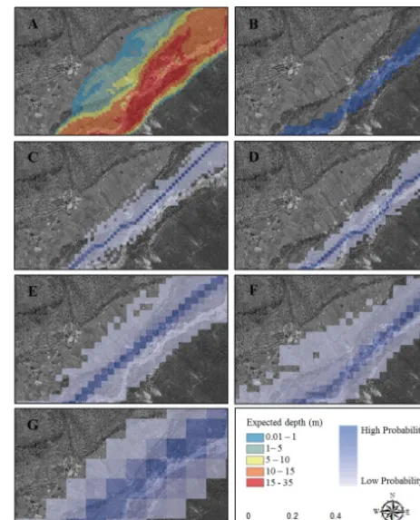
As both the MSF and MC-LCP models have no physical basis, model selection was determined by the one that yielded the most reasonable, conservative estimate of inundation ar-eas when compared to a two-dimensional debris-flow model, FLO-2D, from Imja Tsho (Somos-Valenzuela et al., 2015). Figure 3 shows the flood extent for the FLO-2D, MSF, and MC-LCP models along with the performance of the MC-LCP model for various DEMs (GDEM and SRTM) and resolu-tions (resampled to 15 or 30 m). The comparison revealed the MSF model (Fig. 3b) and the MC-LCP model resampled to a 15 m resolution for the SRTM DEM (Fig. 3c) and the GDEM (Fig. 3d) severely underestimated the flood extent. On the other hand, the MC-LCP model with the 90 m SRTM DEM yielded too conservative an estimate (Fig. 3g). The 30 m results for both the SRTM DEM (Fig. 3e) and GDEM (Fig. 3f) agreed well with the FLO2D results (Fig. 3a); how-ever, a more detailed analysis revealed the GDEM tracked the main channel better. Therefore, the MC-LCP model with the 30m GDEM was used in this study to model the poten-tial GLOFs from each lake. The GLOF from each lake was routed to the confluence of the Sun Kosi for seven of the eight glacial lakes, and approximately 60 km downstream for Thu-lagi Tsho based on the assumption that beyond this distance the downstream effects are minimal as the river is able to ab-sorb the flood’s energy (Vuichard and Zimmermann, 1987). 4.1.6 Downstream impact

Buildings and agricultural land use data were extracted from the inundation extent of each MC-LCP GLOF scenario to provide a first-pass assessment of socio-economic implica-tions. Buildings were downloaded from OpenStreetMap and validated in Google Earth, which was also used to update the data set, when necessary, using the most recent im-agery. Areas of agricultural land were manually digitized in Google Earth and included all visibly managed land, i.e., land that appeared cleared, walled, farmed, or grazed, and would likely have detrimental socio-economic implications if flooded. The potential downstream impact was broken

Figure 3.Inundated areas at Dingboche for a GLOF from Imja Tsho using(a)FLO2D (Somos-Valenzuela et al., 2015), (b) the MSF model using the GDEM, and(c–g)the MC-LCP model with var-ious DEMs and pixel sizes:(c)SRTM 90 m resampled 15 m,(d) GDEM 30 m resampled 15 m,(e)SRTM 90 m resampled 30 m,(f) GDEM 30 m, and(g)SRTM 90 m.

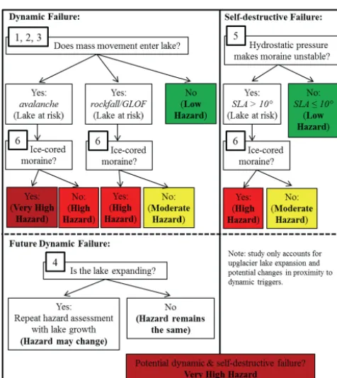
Figure 4.Hazard classification flow chart for determining the haz-ard associated with a glacial lake (numbers refer to hazhaz-ard parame-ters in Fig. 2).

4.2 Risk classification and management actions

The hazard elements described above are crucial for deter-mining whether a glacial lake is susceptible to a dynamic or self-destructive failure. Figure 4 shows the workflow that is used to determine whether the lake is susceptible to failure and how the cause of failure translates into the hazard asso-ciated with the lake. The most dangerous situation is a glacial lake that is susceptible to both dynamic and self-destructive failures, which would classify the lake as a very high haz-ard. Susceptibility is defined as a hazard greater than low; i.e., a lake that is considered a moderate hazard for dynamic failure and a moderate hazard for self-destructive failure is still classified as very high hazard. The other scenario that classifies a lake as very high is a lake with a buried ice core that is susceptible to a snow/ice avalanche, as the ice core may alter the height of the moraine over time and/or the ero-sion and breach of the moraine. A lake that is susceptible to avalanches but does not have an ice core is classified as a high hazard. Snow/ice avalanches were given the highest hazard classification since they are the most frequent cause of failure in the Himalaya (Emmer and Cochachin, 2013). Additionally, any lake with a buried ice core that is suscep-tible to a rockfall or upstream GLOF, or has a steep SLA, is classified as a high hazard. These hazard ratings are meant to reflect self-destructive failures being the second most com-mon cause of GLOFs followed by mass movement entering

Figure 5. Risk management and action framework. Left table: GLOF risk is a function of the hazard and downstream impact. Right table: the recommended course of action for a given glacial lake based on the type of assessment.

the lake from rock or liquid water (Emmer and Cochachin, 2013). As temperatures continue to increase, thereby pro-moting the formation of more glacial lakes and altering slope stability due to changes in permafrost (Haeberli et al., 2016), there is a possibility that failures from rockfalls and/or up-stream GLOFs may become more common than they are in Cordillera Blanca (Emmer and Cochachin, 2013). A lake that does not have an ice core, but is susceptible to a rockfall or upstream GLOF, or has a steep SLA, is considered to be mod-erate hazard.

The risk of a GLOF is a function of a glacial lake’s haz-ard and its potential downstream impact (Fig. 5). This study uses the same ranking scheme as Worni et al. (2013). Very high risk lakes are defined as any lake where the downstream impact is very high; i.e., lives and costly projects are threat-ened, and the hazard of the lake is very high. High risk is defined as a lake that has a high downstream impact and a high hazard, a very high hazard and high/moderate down-stream impact, or vice versa. Moderate risk is defined as a lake that has a moderate hazard and moderate downstream impact, a moderate/low hazard and high downstream impact or vice versa, or a low hazard and very high downstream im-pact or vice versa. Lastly, low risk refers to the remaining scenarios that are less of a threat and is defined as lakes that have a low downstream impact and a low hazard, or a mod-erate hazard and low downstream impact or vice versa. It is important to note that any site that is at risk of a dynamic or self-destructive failure is valuable from an academic perspec-tive as it may help improve the current state of knowledge of GLOF hazards.

5 Results of remote hazard assessment

Table 5.Summary of the hazard parameters for the studied glacial lakes.

Lake Snow/ice Rockfall GLOF SLA (◦) Ice-cored Future change

avalanche upstream moraine to hazards

Chamlang North Tsho Yes Yes No 18.8 No –

Chamlang South Tsho Yes Yes No 10.5 Yes1 –

Dig Tsho Yes Yes No 8.9 No –

Imja Tsho No No No 6.8 Yes1,2 Yes3

Lower Barun Tsho Yes Yes Yes 4.9 Yes1,2 Yes3

Lumding Tsho Yes Yes Yes 10.3 No Yes3

Thulagi Tsho No Yes No 7.1 Yes1,2 No change

Tsho Rolpa Yes Yes Yes 17.5 Yes2 No change

1_{Ponds appear to be on the moraine;}2_{changes in the outlet area identified;}3_{(10–20 years).}

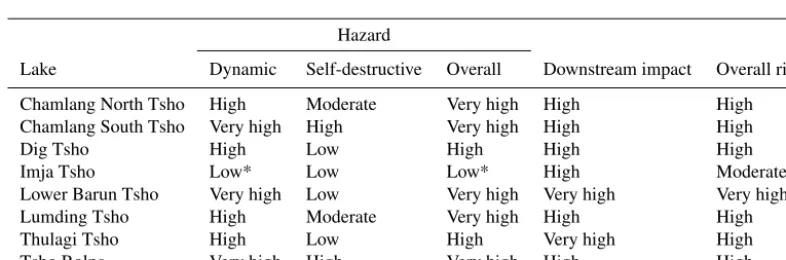
Table 6.Summary of hazard, downstream impact, and risk for each glacial lake.

Hazard

Lake Dynamic Self-destructive Overall Downstream impact Overall risk

Chamlang North Tsho High Moderate Very high High High

Chamlang South Tsho Very high High Very high High High

Dig Tsho High Low High High High

Imja Tsho Low* Low Low* High Moderate*

Lower Barun Tsho Very high Low Very high Very high Very high

Lumding Tsho High Moderate Very high High High

Thulagi Tsho High Low High Very high High

Tsho Rolpa Very high High Very high High High

* Future hazard is very high and risk is high.

scale, which provides valuable information on the potential for mass to enter a lake in addition to identifying the loca-tions of these avalanche- and rockfall-prone areas that should be further investigated. The stability of a moraine utilizes a previously developed approach, i.e., the SLA (Fujita et al., 2013), in combination with predictions of the presence of buried ice from satellite imagery such that self-destructive failures may be integrated into the hazard framework with the dynamic failures. Similarly, the downstream impacts use a previously developed GLOF model, i.e., the MC-LCP ap-proach (Watson et al., 2015), to obtain a conservative esti-mate of potentially inundated areas downstream. For three of the eight glacial lakes considered in this study, this is the first time their potential GLOFs have been modeled. Furthermore, this study combined lake expansion rates from satellite im-agery with ice thickness estimates to model the evolution of these glacial lakes to determine how their hazard may vary over the next 50 years.

Table 5 provides a brief summary of the hazard parame-ters for each glacial lake. The potential for avalanches and rockfalls should not be surprising as these glacial lakes have developed on avalanche-fed debris-covered glaciers, so their surrounding slopes are commonly unstable. Three of the eight glacial lakes are threatened by a potential upstream

GLOF, which makes it important to assess the hazards as-sociated with these upstream lakes as well. The SLA varies between 4.9◦ at Lower Barun Tsho and 18.8◦ for Cham-lang North Tsho. Buried ice is predicted to be present in the moraines of five of these lakes, but only two of these glacial lakes have a SLA above the 10◦threshold, thereby classify-ing these lakes as a high risk of self-destruction.

Figure 6.Area of glacial lakes derived from satellite imagery using the NDWI method from 2000 to 2015 (details in Table S.7).

per km2and percentage of agricultural land affected are ben-eficial for comparing the impacts of different glacial lakes. Tsho Rolpa had the highest amount of affected buildings (56.8 buildings km−2) and agricultural land (16.0 %) fol-lowed closely behind by Thulagi Tsho (49.7 buildings km−2 and 13.1 %, respectively). Chamlang North Tsho, Chamlang South Tsho, and Lumding Tsho had the smallest amounts of inundated buildings and agricultural land affected; however, a GLOF from these lakes could potentially impact on the order of 200 buildings, 2.5 km2of agricultural land, and 15 bridges, which is still cause for considerable concern. Based on these hazard classifications and downstream impacts, the risk for each glacial lake ranged from moderate to very high. These high risk classifications should not be surprising as all the lakes investigated in this study (with the exception of Dig Tsho) were previously deemed hazardous or in need of fur-ther investigation (ICIMOD, 2011; Byers et al., 2013).

Figure 6 shows that Lower Barun Tsho, Imja Tsho, and Lumding Tsho continue to expand rapidly, while Tsho Rolpa and Thulagi Tsho have stagnated in recent years. The other lakes (Chamlang North Tsho, Chamlang South Tsho, and Dig Tsho) have already detached from their glaciers and lack the ability to expand. These expansion estimates combined with the mass movement trajectories reveal that Imja Tsho is susceptible to a dynamic failure in the next 10–20 years (Ta-ble 5). These results have important implications for the haz-ard and risk associated with Imja Tsho as they indicate that in 10–20 years Imja Tsho may be a very high hazard and high risk (Table 6). Additionally, the expansion of Lower Barun Tsho and Lumding Tsho makes them susceptible to potential avalanches located further upstream; however, this does not alter their hazard ratings as they are presently at risk as well.

Figure 7. Hazards and downstream impact for Imja Tsho: (a) avalanche trajectories, (b) rockfall trajectories, (c)ponds on the moraine,(d)future lake expansion, and(e)the extent of the MC-LCP GLOF model(f)highlighting the impacts at Dingboche. The background image(a–e)is Landsat 8 from 30 September 2015 and (f)WorldView 2 from 7 June 2015 (DigitalGlobe, Inc.).

6 Discussion 6.1 Imja Tsho

Imja Tsho is one of the most well-studied glacial lakes in Nepal, yet the remote hazard assessment still yields new rel-evant insight. The mass movement trajectories (Fig. 7a, b) show that the lake is currently not at risk of a dynamic failure. These trajectories are conservative estimates of avalanche and rockfall runout, and for a worst-case scenario they re-main at least 800 and 400 m from the calving front, respec-tively. The ice thickness behind the calving front is greater than 200 m thick (Somos-Valenzuela et al., 2014; Frey et al., 2014), which allows the lake to continue to expand (Fig. 7d). A detailed analysis of the growth of Imja Tsho (Fig. 6) shows the lake is expanding at an average rate of 0.032±0.004 km2yr−1. Based on these expansion rates and the ice thickness estimates, the lake may be at risk of a rock-fall entering the lake in 10 years and an avalanche entering the lake in 20 years.

Table 7.Details of downstream impacts from the MC-LCP GLOF models for each glacial lake.

Total area Buildings Agricultural land Bridges Hydropower

Lake (km2) (total) (km2) (km2) (%) (total) systems

Chamlang North Tsho 28.2 244 8.7 2.5 8.8 14 –

Chamlang South Tsho 27.1 228 8.4 2.5 9.1 14 –

Dig Tsho 30.2 519 17.2 2.8 9.2 23 –

Imja Tsho 32.9 539 16.4 2.7 8.1 28 –

Lower Barun Tsho 45.8 640 14.0 5.9 12.8 20 Yes

Lumding Tsho 25.5 184 7.2 2.4 9.2 16 –

Thulagi Tsho 15.2 754 49.7 2.0 13.1 20 Yes

Tsho Rolpa 49.0 2787 56.8 7.8 16.0 35 –

6.8◦. The melt ponds on the moraine (Fig. 7c) suggest the presence of buried ice, which has been confirmed in the field (Hambrey et al., 2008). The ice-cored moraine is currently not a large concern as its gentle slope does not produce hy-drostatic pressure that endangers the lake. However, satellite imagery reveals the outlet lakes have been changing rapidly, which is important to monitor as these changes may alter the hydrostatic pressure on the moraine (Fujita et al., 2013). If the outlet lakes on the terminal moraine are considered to be part of the lake, the SLA changes to 11.0◦ and Imja Tsho would currently be a high hazard and high risk. Therefore, monitoring the development of the outlet lakes and their in-fluence on the hydrostatic pressure should be a top priority. The MC-LCP model (Fig. 7e, f) shows that 539 buildings and 2.7 km2of agricultural land are at risk (Table 7), which corresponds to a high downstream impact.

Imja Tsho is currently classified as a moderate risk due to its low hazard and high downstream impact. These high downstream impacts highlight the importance of running hy-drodynamic models with high-resolution imagery to improve the mapping of inundated areas and inform the local commu-nities (Somos-Valenzuela et al., 2014). The expansion model reveals that if Imja Tsho continues to grow at its current pace, it will be a very high hazard and high risk in the next 10–20 years. Since the expansion is highly concerning, one important area of future work should be measuring the ice thickness upglacier of Imja-Lhotse Shar Glacier using geo-physical techniques such that the potential future extent of Imja Tsho may be accurately quantified. Additionally, ef-forts should focus on modeling the GLOF process chain, i.e., mass movement entering the lake, the wave propagation, the possible breach of the moraine due to the overtopping, and the downstream impacts due to the future risk. The ice-cored moraine has already been well characterized (Hambrey et al., 2008), but is critical to avoid during any lake lowering activ-ities such that a breach is not initiated. Furthermore, while self-destructive failure is not an immediate concern, repeat bathymetric studies on the outlet lakes would provide valu-able information regarding the evolution of the moraine to understand how the hydrostatic pressures may change over

time. Based on this remote assessment, the current risk mit-igation actions to lower the level of the lake (UNDP, 2013), ideally by 20 m (Somos-Valenzuela et al., 2015), are well jus-tified and hopefully will serve as a good example of how to mitigate the risk of a glacial lake before it becomes highly hazardous.

6.2 Lumding Tsho

Lumding Tsho was classified as a high priority for further in-vestigation (ICIMOD, 2011), but has received very little at-tention beyond an analysis of its expansion (Bajracharya and Mool, 2009) and SLA (Fujita et al., 2013). The remote as-sessment confirms that Lumding Tsho is a very high hazard as it is susceptible to both dynamic and self-destructive fail-ures. The mass movement trajectories reveal the lake is sus-ceptible to avalanches and rockfalls from the southern side slope (Fig. S5a, b). Furthermore, the lake is susceptible to a GLOF from Lumding Tsho Teng located 600 m upstream of Lumding Tsho. Lumding Tsho Teng (27◦47.40N, 86◦37.30E, 5141 m a.s.l.) has an area of 0.34 km2and is susceptible to a large avalanche from its northeastern slope in addition to po-tential rockfalls from its surrounding slopes. Lumding Teng Tsho also has a SLA of 31.7◦, indicating its moraine is highly unstable. These measurements on Lumding Teng Tsho indi-cate the lake is a very high hazard, so an upstream GLOF should be a great concern for Lumding Tsho.

in-Figure 8.Bathymetric survey conducted on Lumding Tsho on 22– 23 October 2015.

creases, but its hazard classification does not change as it is already classified as a very high hazard. The MC-LCP GLOF model (Fig. S5e, f) reveals 184 buildings and 2.0 km2of agri-cultural land are at risk (Table 7). This downstream impact is the smallest of those considered in this study, but still shows there is considerable risk to livelihoods downstream, thereby classifying Lumding Tsho as high risk.

An initial rapid reconnaissance was undertaken from 20 to 24 October 2015 to assess the hazards associated with Lumd-ing Tsho as directed by the management action framework (Fig. 5). The short field campaign consisted of a bathymet-ric study, streamflow measurements of the outlet, and visual inspection of the terminal moraine and surrounding slopes. The bathymetric survey was conducted over 2 days using an inflatable kayak and a Garmin echoMAP 54dv to mea-sure 4768 points of lake depth. The shoreline was delineated using the NDWI methods as previously reported. The shore-line was converted into point measurements that were used in conjunction with the bathymetric survey to interpolate depth throughout the lake using the Topo to Raster tool in ArcGIS (Somos-Valenzuela et al., 2014). The lake was found to have an average depth of 51 m, a maximum depth of 114 m, and a total volume of 57.7×106m3(Fig. 8).

Streamflow from the outlet of the lake was measured to be 8.4 m3s−1in the afternoon of 23 October using a Pygmy Current Meter with an AquaCalc Pro Plus computer (Rickly Hydrological Company). Inspection of the terminal moraine revealed the outlet was the only source of water exiting the lake; i.e., there was no apparent seepage through the terminal moraine. Additionally, no ponds or karst-like features were present on the terminal moraine, which further indicated that the moraine was relatively stable. In contrast to the SLA, the terminal moraine appeared to be relatively gentle and fairly wide (Fig. 9c). A detailed analysis of the SLA calculations reveals there is a large waterfall located 1 km downstream of

Figure 9.Lumding Tsho and its surrounding slopes with areas of concern highlighted in red showing(a)the calving front and prone areas behind the glacier,(b) the southern side slope, and(c) the terminal moraine and its gentle outlet.

Lumding Tsho. If the distance from the lake used to com-pute the SLA was changed from 1 km to 950 m, then the SLA changes to 9.8◦_{, which would change the hazard of a}

potential self-destructive failure from moderate to low. The waterfall is important to consider as this drop in elevation would generate a significant amount of energy that could ex-acerbate a GLOF downstream. Therefore, a physically based flood model that can account for this acquisition of energy would be valuable for improving estimates of the potential downstream impacts.

glacial lake, was unable to be conducted. Similar knowledge of the stability of the slopes surrounding Lumding Teng Tsho would inform the likelihood of an upstream GLOF. A bathy-metric study on Lumding Teng Tsho and an assessment of the stability of its moraine should also be a high priority. In the event of a GLOF, the northern lateral moraine of Lumd-ing Tsho may or may not protect the lake from the upstream flood. A physically based GLOF model that accounts for erosion would yield insight into the potential breach of the lateral moraine and subsequent GLOF from Lumding Tsho. Based on the rapid field reconnaissance, the hazard associ-ated with Lumding Tsho can be reduced from very high to high due to the apparent stability of the moraine. However, more detailed analyses of slope stability around Lumding Tsho and Lumding Teng Tsho in addition to modeling the potential GLOFs from both of these lakes should be a top priority.

6.3 Chamlang North Tsho

Chamlang North Tsho has already reached its fullest extent, so its proximity to hazards is not going to change over time (Fig. S1d). The southern and eastern slopes reveal the lake is very susceptible to rockfalls and avalanches to the extent that any rockfall or avalanche will enter the lake (Fig. S1a, b). This potential for a dynamic failure is exacerbated by its steep terminal moraine, which has a SLA of 18.8◦. This SLA is the highest among the eight glacial lakes investigated in this study and much greater than the stability threshold of 10◦. Fortunately, no melt ponds were observed on the moraine and the outlet appears to be stable from satellite im-agery, indicating an ice-cored moraine is unlikely (Fig. S1c). Nonetheless, the combination of the steep terminal moraine and the likelihood of mass movement entering the lake give Chamlang North Tsho a classification of a very high haz-ard. The MC-LCP GLOF model (Fig. S1e, f) reveals that 244 buildings and 2.5 km2of agricultural land are at risk (Ta-ble 7), causing Chamlang North Tsho to be a high risk.

Based on the remote assessment, the most important area of future investigation should be modeling the GLOF pro-cess chain. The avalanche-prone slopes were observed by Byers et al. (2013), who identified four overhanging glaciers on Chamlang North Tsho’s southern slopes. The use of high-resolution imagery may help quantify the size of a po-tential avalanche. Byers et al. (2013) modeled a popo-tential GLOF using the GDEM with the U.S. Army Corps of En-gineers’ Hydrologic Engineering Center River Analysis Sys-tem (HEC-RAS). The ensuing flood model provides an im-proved estimate compared to the MC-LCP model, which es-timates the water level will rise by 9 m at Bung; however, the downstream impacts were not detailed due to the lack of high-resolution imagery. The acquisition of high-resolution DEMs for this region and/or cross sections at critical loca-tions should be a high priority. This high-resolution DEM should be used with two-dimensional flood models to more

accurately estimate the downstream impacts. Additionally, a geotechnical survey including sedimentological sampling of the moraine should be performed such that erosion can be properly accounted for in breach scenarios (Westoby et al., 2015) and the stability of the moraine with respect to the current hydrostatic pressures may be quantified. Lastly, a bathymetric survey of Chamlang North Tsho is needed for the high-resolution physically based GLOF modeling. 6.4 Chamlang South Tsho

Chamlang South Tsho has very similar hazard characteris-tics to Chamlang North Tsho. Chamlang South Tsho is no longer expanding as it has already reached its fullest extent (Fig. 6). Mass movement trajectories also show that the lake is surrounded by unstable slopes such that any rockfall or avalanche will enter the lake (Fig. S2a, b). The SLA ex-ceeds the stability threshold with a value of 10.5◦_,

indicat-ing that the moraine is unstable. Additionally, satellite im-agery reveals the presence of melt ponds on the moraine, thereby suggesting the moraine is ice-cored (Fig. S2c), which has been verified from the differencing of multi-temporal high-resolution DEMs (Sawagaki et al., 2012; Lamsal et al., 2016). Therefore, the steep ice-cored moraine is considered to be a high risk for self-destruction. The combination of self-destructive failure and the potential for a dynamic fail-ure classifies this glacial lake as a very high hazard. The MC-LCP GLOF model (Fig. S2e, f) also reveals 228 build-ings and 2.5 km2of agricultural land are at risk (Table 7), so Chamlang South Tsho is considered to be a high risk.

These conflicting studies, which had access to the same data and had similar on-site observations, highlight the need to take an objective approach towards understanding the risks associated with a glacial lake. The main priority with re-spect to Chamlang South Tsho should be modeling the en-tire GLOF process chain. This objective analysis would clar-ify the conflicting views on the potential for a dynamic fail-ure. As a first-pass approach, the methods used by Heller and Hager (2010) were applied to estimate the impulse wave height using one of the avalanche volumes and tracks from the mass movement modeling. The modeled avalanche was 8.1×104m3 (assumed 10 m thickness) located 800 m east of Chamlang South Tsho at an elevation of 5650 m a.s.l. The avalanche density was assumed to be 500 kg m3 and the avalanche was assumed to expand from its initial width of 90 m to the width of the lake at the location where the avalanche enters the lake (300 m). Based on these assump-tions, the avalanche would generate a 20.5 m wave, which would likely easily overtop the ice-cored moraine. This sim-plified approach highlights the importance of using high-resolution satellite imagery to determine the potential sizes of avalanches in conjunction with physically based models to more accurately model the avalanche, the wave propagation, and any potential overtopping and/or breaching that may oc-cur.

Additionally, the potential for a self-destructive failure needs to be explored in further detail as the remote assess-ment suggests the lake is unstable, which is supported by the SLA calculations in Fujita et al. (2013) and the observations and measurements from Lamsal et al. (2016). A chemical analysis of the seepage would lend insight as to the source of the water, i.e., whether the water is the melting of the ice core or lake water. Geophysical surveys of the terminal moraine should be used to determine the spatial extent and depth of the ice core and geotechnical surveys of the composition of the debris would be valuable for assessing the stability of the moraine in detail. Lastly, Lamsal et al. (2016) highlighted the potential downstream impact and Byers et al. (2013) noted that a GLOF from Chamlang South Tsho is a concern for these communities, so improved modeling using a physically based GLOF model should be a top priority. The combina-tion of these modeling efforts and field measurements would definitively determine the hazard of the lake and the threat to downstream communities.

6.5 Dig Tsho

Dig Tsho is a prime example of why glacial lakes should not be prioritized based on the size of the lake. In 1985, Dig Tsho was only 0.5 km2 with a maximum depth of 18 m, yet its GLOF had devastating impacts downstream (Vuichard and Zimmermann, 1987). The breach of its moraine reduced the lake to its present size of 0.4 km2 (Fig. 6). The remote as-sessment shows that Dig Tsho is still very susceptible to an-other dynamic failure (Fig. S3a, b), as any mass movement

from the surrounding slopes is likely to enter the glacial lake. Fortunately, its previously breached moraine appears to be very stable as its SLA is 8.9◦_{, and an ice core is unlikely}

(Fig. S3c). Based on the potential for another dynamic fail-ure, Dig Tsho is classified as a high hazard. The MC-LCP model (Fig. S3e, f) shows that 519 buildings and 2.8 km2are at risk from a GLOF (Table 7), thereby classifying Dig Tsho as a high risk based on the remote assessment.

Field investigations should assess the current bathymetry of the lake to determine the amount of water that could be displaced by a GLOF. Most likely the maximum depth greatly diminished after the GLOF in conjunction with the reduction in the area of the lake, so the potential GLOF discharge would be smaller than the 1985 GLOF. A one-dimensional GLOF model that has been applied to other glacial lakes in Nepal (Byers et al., 2013; Khanal et al., 2015) would be beneficial in determining how the downstream im-pacts have changed based on the new bathymetry.

6.6 Lower Barun Tsho

be at risk (Table 7). Therefore, Lower Barun Tsho has a very high downstream impact and is classified as a very high risk. Similar to Lumding Tsho, Lower Barun Tsho should be a main priority of future field campaigns in Nepal as the lake is a very high risk, but has received little attention. Field campaigns should focus on investigating the potential of mass movement entering the lake from the southern slopes of Lower Barun Tsho. This investigation should be coordi-nated with physically based modeling efforts of the GLOF process chain to determine how mass movement entering the lake will propagate across the lake and potentially breach the moraine. While the lake is unlikely to fail due to the hydro-static pressures, a sedimentological survey of the composi-tion of the moraine would greatly improve modeling a poten-tial breach. Geophysical techniques should also be performed on the moraine to determine the presence and spatial extent of the potential ice core as this may have large implications on the breach of the GLOF. The expansion of Lower Barun Tsho is a large concern as it only increases its susceptibility to rockfall and avalanche-prone areas upglacier; therefore, geophysical techniques should be used on Barun Glacier to determine the maximum potential extent of the glacial lake. Additionally, bathymetric surveys should be performed on Lower Barun Tsho to aid modeling efforts of the GLOF pro-cess chain. Seto Pohkari also requires attention with regard to its bathymetry and modeling the process chain for avalanches and rockfalls from its surrounding slopes. Similar to Lumd-ing Tsho, the northern lateral moraine of Lower Barun Tsho may protect the lake from the upstream GLOF. Therefore, a physically based flood model for both Lower Barun Tsho and Seto Pohkari would greatly improve the understanding of the risk faced by downstream communities.

6.7 Thulagi Tsho

Thulagi Tsho is one of the three glacial lakes where field campaigns were performed to investigate the hazard of a GLOF by ICIMOD (2011). The results from the remote as-sessment yield valuable information that may be used to sup-plement these initial field campaigns. Mass movement tra-jectories reveal the lake is susceptible to rockfalls from both side slopes but is not susceptible to avalanches (Fig. S6a, b). Figure 6 shows that the lake growth has stalled since 2010. The lake expansion model reveals the bed elevation of the glacier behind the calving front is greater than the lake level, indicating that the lake may have reached its maximum spa-tial extent (Fig. S6d). An assessment of the terminal moraine shows there are ponds on the terminal moraine and the out-let channel has changed in the last 15 years, which suggests the moraine is ice-cored. Fortunately, the SLA of 7.1◦ re-veals the terminal moraine is apparently stable. This finding is in direct contrast to Fujita et al. (2013), which estimated a potential flood volume for Thulagi Tsho of 0.6 million m3, indicating the SLA was greater than the 10◦threshold. These differences are likely due to the 100 m buffer, the exclusion

of the melt ponds, and/or potential differences in the lake delineations and DEMs used in this study. Based on this analysis, the lake is a high hazard due to the chance of a dynamic failure in conjunction with the ice-cored moraine. The MC-LCP GLOF model (Fig. S6e, f) reveals 754 build-ings, 2.0 km2of agricultural land, and planned hydropower projects (ICIMOD, 2011) are at risk (Table 7). These down-stream impacts were among the most severe of the glacial lakes in this study, as shown by the second highest number of buildings per km2and percentage of agricultural land. The combination of these very high downstream impacts and high hazards classify Thulagi Tsho as a high risk.

As previously mentioned, the results of the remote assess-ment provide valuable information to suppleassess-ment the work performed by ICIMOD (2011) and the one-dimensional GLOF modeling performed by Khanal et al. (2015). Specif-ically, the lake expansion model shows that Thulagi Tsho appears to have reached its maximum extent, which should be confirmed with a geophysical survey measuring ice thick-ness behind the calving front. Additionally, the mass move-ment trajectories are the first time any slope stability has been modeled at this site. These trajectories reveal the lake’s vul-nerability to mass movement entering the lake and should be the focus of future modeling efforts at this lake. High-resolution satellite imagery and field inspection should be used to determine the potential size of any rockfall such that these estimates may be applied to a physically based mass movement model. These mass movement models could be used in conjunction with the bathymetric survey by ICI-MOD (2011) to model the wave propagation and breach of the moraine. A sedimentological survey to accompany the geophysical investigations performed by ICIMOD (2011) would allow the moraine stability and breach parameters to be quantified with greater accuracy. Furthermore, Khanal et al. (2015) also found the downstream impacts from a GLOF were very high; therefore, a two-dimensional physi-cally based model should build off these results to more ac-curately quantify the risks and vulnerable areas, which may be used to inform the downstream communities.

6.8 Tsho Rolpa

finding. If the model is correct, this has large implications for the hazard of the lake, as this will limit the magnitude of future avalanches entering the lake; i.e., Richardson and Reynolds (2000) found that the magnitude of avalanches was increasing as the lake grew. The mass movement trajectories show that the lake is susceptible to avalanches from its north-ern slope (Fig. S7a) and rockfalls from its surrounding side slopes (Fig. S7b). The avalanche activity has been a major concern for Tsho Rolpa, so the logical next step is to use physically based models to model the GLOF process chain and determine how vulnerable the lake is to these threats. Satellite imagery from the last decade also reveals changes in the islands near the terminal moraine, which suggest the presence of an ice core (Fig. S7c). The ice core has been confirmed and well documented (ICIMOD, 2011). Addition-ally, the SLA of 17.5◦ is the second highest of any of the glacial lakes in this study and Fujita et al. (2013) found Tsho Rolpa had the highest potential flood volume of the lakes in their study. The combination of the ice core, the high SLA, and the potential for mass movement to enter the lake con-firms the previous assessments that Tsho Rolpa is a very high hazard.

Additionally, there are three glacial lakes located upstream that are threats to Tsho Rolpa. The first upstream glacial lake, Tsho Rolpa Upper 1 (27◦50.70N, 86◦27.80E, 4968 m a.s.l.), is located 1.5 km southeast of Tsho Rolpa and has an area of 0.12 km2. The hazard assessment reveals this upstream glacial lake is susceptible to ice avalanches and rockfalls, and has a SLA of 13.0◦, thereby classifying Tsho Rolpa Upper 1 as a high hazard. The MC-LCP model reveals a GLOF has the potential to enter Tsho Rolpa; however, this would re-quire the upstream GLOF to overtop and/or erode the south-ern lateral moraine of Tsho Rolpa. Similar to Lumding Tsho and Lower Barun Tsho, flood modeling that incorporates erosion would help determine whether this lake is a cred-ible threat to Tsho Rolpa. The second glacial lake located upstream of Tsho Rolpa, Tsho Rolpa Upper 2 (27◦50.10N, 86◦29.00E, 4858 m a.s.l.), has an area of 0.03 km2and is only susceptible to potential rockfalls. It also has a SLA of 10.1◦, thereby classifying the lake as a very high hazard. The third glacial lake, Tsho Rolpa Upper 3 (27◦51.40N, 86◦30.00E, 5316 m a.s.l.), has an area of 0.02 km2and is also only sus-ceptible to potential rockfalls. This lake has a greater SLA of 20.2◦, which also classifies it as a very high hazard. How-ever, while Tsho Rolpa Upper 1 is much larger and appears to be a greater hazard than the other two upstream glacial lakes, the MC-LCP GLOFs reveal a GLOF from Tsho Rolpa Upper 2 or 3 would flow onto Trakarding Glacier and directly en-ter Tsho Rolpa. Therefore, the hazard associated with these glacial lakes should be further investigated.

The MC-LCP GLOF model of Tsho Rolpa (Fig. S7e, f) shows that 2787 buildings, 7.8 km2of agricultural land, and 35 bridges would be at risk (Table 7). These impacts are both the highest number of buildings per km2 affected and the highest percentage of agricultural land affected, which

classi-fied the risk associated with Tsho Rolpa as very high. Khanal et al. (2015) used a one-dimensional model, which confirmed the severe consequences downstream and highlights the im-portance of applying a two-dimensional model to create ac-curate hazard maps for the communities. This assessment is in agreement with other studies that Tsho Rolpa is still a high risk despite the fact that the lake was lowered by 3–4 m. Those risk-mitigation efforts serve as a good example that lowering the level of these lakes is possible, but also high-lights the need to lower the lake 15–20 m further (Reynolds, 1999). A detailed analysis of the changes in the GLOF as a function of the lowered lake level would be a valuable re-source to determine the exact amount the lake should be low-ered.

7 Conclusions

The remote assessment integrates the key hazard parameters in an objective manner that is repeatable and relies solely on globally available remotely sensed data. This study investi-gated eight glacial lakes in Nepal that are widely considered to be highly hazardous and was found to yield valuable in-sight with respect to each lake regardless of the amount of previous attention the lake had received. For Lumding Tsho and Lower Barun Tsho, this was the first time these lakes have been holistically studied since they were listed as a high priority of further investigation. For other glacial lakes that have already been studied extensively, e.g., Tsho Rolpa and Imja Tsho, the remote assessment yielded valuable in-formation regarding their future expansions. This study is the first of its kind to incorporate detailed modeling of lake growth into a hazard assessment. For Imja Tsho this is par-ticularly valuable as the assessment is able to identify future hazardous conditions before they occur and hopefully shows the benefit of implementing risk-mitigation strategies prior to the lake becoming highly hazardous.