Passive acoustic measurement of bedload grain size distribution
using self-generated noise
Teodor Petrut1,2, Thomas Geay1, Cédric Gervaise4, Philippe Belleudy2, and Sebastien Zanker3 1Université Grenoble Alpes, Grenoble INP, CNRS, GIPSA-Lab, 38402 Grenoble, France
2Université Grenoble Alpes, CNRS, IRD, Grenoble INP, IGE, 38058 Grenoble, France 3Électricité de France, DTG division, Grenoble, 38040, France
4Institut de recherche CHORUS, Phelma Campus, 38000 Grenoble, France Correspondence:Teodor Petrut ([email protected])
Received: 22 March 2017 – Discussion started: 22 May 2017
Revised: 17 November 2017 – Accepted: 6 December 2017 – Published: 26 January 2018
Abstract.Monitoring sediment transport processes in rivers is of particular interest to engineers and scientists to as-sess the stability of rivers and hydraulic structures. Various methods for sediment transport process description were pro-posed using conventional or surrogate measurement tech-niques. This paper addresses the topic of the passive acous-tic monitoring of bedload transport in rivers and especially the estimation of the bedload grain size distribution from self-generated noise. It discusses the feasibility of linking the acoustic signal spectrum shape to bedload grain sizes involved in elastic impacts with the river bed treated as a massive slab. Bedload grain size distribution is estimated by a regularized algebraic inversion scheme fed with the power spectrum density of river noise estimated from one hydrophone. The inversion methodology relies upon a phys-ical model that predicts the acoustic field generated by the collision between rigid bodies. Here we proposed an ana-lytic model of the acoustic energy spectrum generated by the impacts between a sphere and a slab. The proposed model computes the power spectral density of bedload noise using a linear system of analytic energy spectra weighted by the grain size distribution. The algebraic system of equations is then solved by least square optimization and solution regular-ization methods. The result of inversion leads directly to the estimation of the bedload grain size distribution. The inver-sion method was applied to real acoustic data from passive acoustics experiments realized on the Isère River, in France. The inversion of in situ measured spectra reveals good esti-mations of grain size distribution, fairly close to what was estimated by physical sampling instruments. These results
il-lustrate the potential of the hydrophone technique to be used as a standalone method that could ensure high spatial and temporal resolution measurements for sediment transport in rivers.
1 Introduction
en-hances the accuracy of transport rate prediction. Therefore, measuring bedload leads to not only transport rates, but also to bedload GSD to calibrate models (Parker, 2002; Wilcock et al., 2009). However, obtaining bedload samples during ex-ceptional hydraulic events may be difficult by using tradi-tional bedload sampling techniques (e.g., pressure-difference samplers) (Bunte et al., 2010). To measure a wide range of discharge flows, the scientific community has been interested in developing indirect, or surrogate, methods that achieve continuous measurements no matter the hydraulic conditions (Gray et al., 2010; Hubbell, 1964). This paper is dedicated to the monitoring of bedload GSD using the acoustic noise nat-urally generated by bedload transport in rivers, the so-called bedload self-generated noise (SGN).
Acoustics surrogate methods are divided into two cat-egories: active and passive methods (Gray et al., 2010; Hubbell, 1964). Examples of active methods are the acoustic Doppler current profiler, aDcp (Rennie and Millar, 2004), or the acoustic mapping velocity technique (Muste et al., 2016). Active methods use emissions of well-known signals but, ac-tually, to the best of our knowledge, no active instrument was conceived to estimate bedload GSD. Besides, the major prob-lem of the active instruments is that they do not properly be-have during high flow discharges. This is why the passive instruments are preferred instead of the former. These in-struments use seismic or acoustic signals generated by bed-load particle impacts. Recorded signals contain information on both sediment impact rate and bedload particle sizes. One of the most widely used techniques consists in recording the signal of particle impacts on steel objects like plates (Rick-enmann et al., 2014; Wyss et al., 2016a), pipes (Mao et al., 2016; Mizuyama et al., 2010) or column pipes (Papanicolaou et al., 2009). Other passive instruments consist in directly recording bedload SGN by using passive acoustic monitor-ing (PAM) (Barton, 2006; Bedeus and Ivicsis, 1963; Geay, 2013; Geay et al., 2017a; Thorne, 1986a, b) or seismic mon-itoring (Gimbert et al., 2014; Roth et al., 2016; Tsai et al., 2012). Measuring bedload GSD with passive methods has been achieved using plates (Barrière et al., 2015; Krein et al., 2014; Rickenmann et al., 2014; Wyss et al., 2016b) or pipes (Dell’Agnese et al., 2014; Mizuyama et al., 2010; Papani-colaou et al., 2009), and SGN (Geay et al., 2017a; Johnson and Muir, 1969; Jonys, 1976; Thorne, 1986a, b), by using experimental laws of calibration. Concerning seismic meth-ods, bedload GSD measurements were not yet proposed as a direct application.
The existence of a link between the GSD and the features of vibrational signals has been demonstrated in several exper-iments (Belleudy et al., 2010; Bogen and Møen, 2001; Krein et al., 2008; Turowski et al., 2011). Coupling geophones with steel plates (Barrière et al., 2015; Wyss et al., 2016a) pro-duced composite power laws by linking both peak ampli-tude and peak frequency to the grain size. Using the Japanese pipe, Mao et al. (2016) proposed an empirical model based on multi-channel recorded amplitude ratios to estimate
dif-ferent percentiles of grain diameters (D16, D50 andD84). The only metric exploited in this kind of measurement is the amplitude of shocks on steel structures. Thus, these passive techniques involving shocks on steel structures offer a high-quality signal, or signal-to-noise ratios (SNRs). The analyzed physics is the same as in the case of SGN measurements by PAM, which is the rigid body radiation caused by Hertzian impacts between sediments. In the case of SGN measure-ments, unlike the steel structure impact measuremeasure-ments, the SGN signal amplitudes are not usable for grain-size inver-sion because of the issues concerning the sound propagation throughout the reach (the amplitudes depend on the distance between the shocks and the hydrophone). This makes the am-plitude a futile metric to infer grain-size information from SGN signals.
Several studies in the field highlighted that the frequency content (i.e., spectrum shape) of SGN signals is heavily dom-inated by grain sizes. For example, Jonys (1976) showed by laboratory experiments with ceramic spheres that spec-tral peak frequency is linked to sphere diameter. The author found a peak frequency at about 4 kHz for 19 mm diameter particles, at 2.2 kHz for the 38 mm diameter and at 1 kHz for the 75 mm diameter. This means that a doubling of grain size is almost equivalent to halving of peak frequency. Extensive research on GSD estimation by SGN recordings was done by Thorne (1986b), where he presented two strategies for in-version of acoustic spectra to estimate GSD. Results were encouraging as GSD was roughly estimated. These tech-niques are based on experimental measurements that have been made in a rotating drum with specific conditions that are different from the conditions found in rivers (e.g., impact velocities, acoustic propagation). Besides, his inversion tech-niques raise issues because of the broadband nature (shape) of spectra, even for uniform sediments. The author himself assumed that this was the major cause of inaccurate estima-tions of GSD from composite spectra.
tween a sphere and a slab (Akay and Hodgson, 1978; Hunter, 1957), because the main assumption of this study is that the acoustics of gravel is described by impacts between bedload sediments and the river. To prove the validity of our model, the study includes some comparative facts with the sphere– sphere spectral model of Thorne and Foden (1988).
As a brief introduction, the collision between bed particles radiates energy. Such a rigid body radiation phenomenon is due to both vibrations and accelerations. These processes are very well separated with respect to their dominant frequen-cies, such that the spherical mode vibrations generate much higher frequencies than the acceleration-based sound (Bar-ton, 2006; Thorne and Foden, 1988). The acoustic effect of accelerating rigid bodies is physically modeled by Kirchhoff (1883). A framework was constructed by Goldsmith (2003), Hertz (1882) and Hunter (1957) to model acceleration pro-files from elastic impacts between two solid rigid bodies like two spheres or a sphere and a slab. In a mathematical sense, the acoustic pressure field generated from the acceler-ation of a rigid body is evaluated by the integral convolution from Eq. (1) (Akay and Hodgson, 1978; Koss and Alfred-son, 1973; Thorne and Foden, 1988). The integral consists of the convolution between Kirchhoff’s impulse responsepI and an acceleration profile A. In the case of elastic (Hertzian) impacts the acceleration occurs during the impact, and so the integral is evaluated by intervals with respect to a contact du-rationTc. The contact durationTcis modeled by Hertz’s law and it is put in a simplified form in Eq. (2), for both sphere– sphere and sphere–slab impact models.
p(t )= χ
Z
0
pI(t0)·A(t−t0)dt0, (1)
Tc=ϑ(1)(ζ ρs)0.4aUimp−0.2, (2) whereχ is the time interval of convolution, withχ=t, if 0 ≤τ ≤Tc, andχ=Tc, ifτ > Tc, withτ a delayed time due to sphere geometry,τ =t−(r−a)/c,ris the distance between the observation point and the impact (see also Fig. 1a and b),
ais the radius of the sphere,cis the sound celerity,ρsis ma-terial density andUimpis the impact velocity. The parameter
ϑ(1)is a constant,ϑ(1)=9.229, for the impact between two spheres of the same radii andϑ(1)=10.601, for the impact of a slab and a sphere. The parameterζ =(1−ν2)/(π Elong) is a material parameter, and it contains Young’s modulus (Elong) and the Poisson ratio (ν).
The general form of the acceleration profile is provided by Goldsmith (2003) and it is rewritten in a unified form for both
andϑ(2)=3.353 for sphere–slab impact.
The first important observation from Eq. (3) is the half-period sinusoidal form of the Hertzian acceleration. The two modeled acceleration laws show close frequencies as the constantϑ(1)fromTc’s formula is not dramatically different from one case to another. If the frequency of acceleration of sphere–sphere impact is 1000 Hz, then the frequency of ac-celeration of sphere–slab impact is 909 Hz, which is almost only 10 % of the deviation. The maximum amplitude of ac-celeration for the impact between two spheres of radiusais almost 2 times less than the impact between a sphere of ra-diusaand a slab, considering the sameUimpandTc.
The integral convolution in Eq. (1) is transformed into multiplication in the complex Fourier space. Thus, the an-alytical magnitude spectrum of the noise from the rigid body acceleration,Facc, is given in Eq. (4a).
Facc(ω)=F (pI(t ))·F (A(t )), (4a) whereF (pI)is the Fourier transform (FT) of Kirchhoff’s im-pulse responsepI(Koss and Alfredson, 1973), for a sphere of radiusa, defined in Eq. (4b),F (A)the FT of Hertzian ac-celeration due to elastic impact between two identical radii and the same material spheres, defined in Eq. (4c), andωis the angular frequency which is a measure of rotation rate, in radians per seconds, and it is equal to 2πf;f is the linear frequency, a measure of number of occurrences per second.
F (pI)= ρa3c
r2 (c+j ωr)
2c2−(ωa)2−j2ωac
2c2−(ωa)22
+(2ωac)2
cosθ (4b)
F (A)=ϑ(3) U π2−(ωT
c)2
e−j ωTc+1 (4c)
j is an imaginary unit andϑ(3)= ±π2/2 for sphere–sphere impact, andϑ(3)=1.067π2for sphere–slab impact.
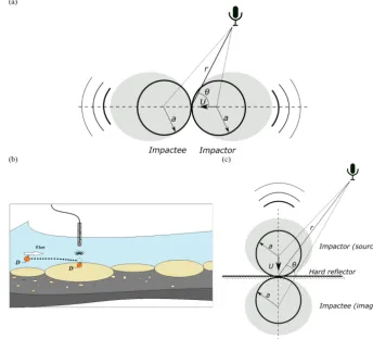
Figure 1. (a)Setup for the impact between two spheres, here of the same radiusa; the acoustic dipole source is illustratively depicted by the gray patch;(b)setup for the impact between a sphere of radiusaand a semi-infinite rigid plane; to be noted is the boundary condition of the hard bottom (reflector) assumed in the framework of the “method of images”; thus, the impacting sphere is mirrored in the slab, so the acoustic fields are subtracted; the acoustic dipole source is illustratively depicted by the gray patch;(c)the elementary acoustic process of bedload noise in the river: the particle of equivalent diameterD=2aimpacts the armored river bed (a massive slab) which generates a transient recorded by a hydrophone.
Table 1.Parameters used to model analytical spectra of sediment size mixtures, Eq. (9b), and the typical values adapted for the underwater environment. The typical singular values are used in inversion further in this paper. The ranges of values are used in the global sensitivity analysis.Kis the number of size classes used to inverse acoustic spectra.
Parameters Typical range of Typical Units Remarks values in under- values used
water medium in inversion
Particle diameter (D) 0–150 {1,2, . . .,150} mm D50is used in the global sensitivity analysis (GSA). SD (σ) 0.01–10 2D50=D84 mm Used in the GSA; the relation 2D50=D84is typically
used (Recking, 2013).
Impact velocity (Uimp) 0.001. . .5 {0.01; 0.1; 1; 5} m s−1 The same for all the grain size classes
Distance of measurement (r) 0.01. . .10 1 m It acts on the delay timeTdfound in the model of Eq. (7). Angle of directivity (θ) 0◦. . .90◦ 0◦ deg In theory, ifθ=90◦, then the wave amplitude is
zero; it also defines theTd.
Sound celerity in water (c) 1403–1507 1483 m s−1 Dependent on temperature, water salinity, etc. Water density (ρ) 960–1025 999 kgm−3 Dependent on temperature, water salinity, etc. Modulus of elasticity (Elong) 10–70 55 GPa Materials like limestone, quartz, or granite. Poisson’s ratio of impacting 0.15–0.2 0.2 − The typical values are for granite. bodies (ν) The densityρsis used to
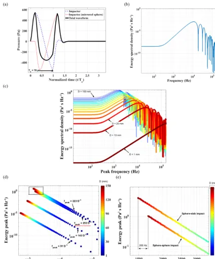
[image:4.612.49.546.514.700.2]Figure 2. (a)Analytical waveform of sound from impact between a granite sphere of diameterD=20 mm and a granite slab, where the impact velocityUimp=1 m s−1, the directivity angleθ=0◦ and the sensor isr=1 m from the impact; the arrow indicates the contact durationTd;(b) the analytical spectrum modeled with Eq. (7) using the same parameters as in(a); the spectrum is an energy spectral density and is measured in Pa2s Hz−1;(c)analytical spectra of sphere–slab impacts modeled by Eq. (7) as a function of diameter,D= {1,10,20,30. . .150}mm; impact velocityUimp=1 m s−1, the directivity angleθ=0◦and the sensor isr=1 m from the impact.(d)Peak frequencyfpeak and power peak variations, from spectra modeled by Eq. (7), with the diameter and the sphere’s diameters; the diameters are coded by colors. The power lawfpeak=aDb is given, where the sphere–slab impact tests consider three impact velocities (Uimp=
{0.01,0.1,1}m s−1) and the law of sphere–sphere impact is underlined by the dotted line; the material is granite. From bottom to top, the regression laws of sphere–slab impact vary fromUimp=0.01 (bottom) toUimp=1 (top) m s−1. The sphere–sphere impact tests are done usingUimp=1 m s−1and the same other parameters as with sphere–slab impacts.(e)Detail where the two vertical dotted lines locate the
[image:5.612.86.510.66.577.2]Figure 3.GSA flowchart to compute the first-order sensitivity indices by the FAST method; the spectrum is simulated with Eqs. (7) and (9b), with a log-normal distribution generated using a diameter in the range 1 to 150 mm and SDσ in the range 0.01 to 10. The rest of the input parameters are defined in Table 1. From the simulated spectra, thefpeakare computed, and finally the first-order sensitivity indicesSi are
calculated using the FAST method. The results are shown in Table 2.
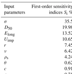
Table 2. First-order sensitivity indicesSi computed by the FAST
method, assuming the peak frequency as the output of the model,
fpeak: 0 % means no influence, and 100 % means total influence on the model output.
Input First-order sensitivity parameters indicesSi%
σ 35.5
D50 19.98
Elong 13.52
Uimp 10.65
r 7.45
ν 6.42
ρs 4.24
θ 0.62
c 0.91
ρ 0.71
in phase), so there are two waves (compression and rarefac-tion) arriving at the sensor almost at the same time (Akay and Hodgson, 1978). This acoustic process is modeled by the so-called method of images by which one considers a mirrored sphere replacing the slab and being responsible for the rar-efaction wave generation.
The same subtraction is applied in the case of complex spectra to obtain the total spectrumFim, Eq. (5). In this for-mula, the first term of the right member is attributed to the impacting sphere, whereas the second term pertains to the mirror. The time delayTdof sound arrival due to distance of measurement and the sphere’s geometry make the two terms not perfectly cancel out or not arrive at the same time at the sensor.
Fim(ω)=Facc(ω)−Facc(ω)·e−j ωTd (5) Introducing Eqs. (2), (3) and (4a–c) into Eq. (5), one ob-tains the complex magnitude spectrum of the impact between a sphere and a slab. The spectrum contains complex numbers, so one applies the multiplication of the spectrum and its con-jugate to compute the magnitudes of the energy spectrum, Eq. (6).
|Fim|2=Fim·Fim∗, (6)
whereFim∗ is the complex conjugate ofFim.
The quantity |Fim|2 from Eq. (6) is noted as in Eq. (7) by E and its unit of measurement is Pa2s Hz−1. Thus, the
analytical model of impact used in this paper is an energy spectral density and it will be used to inverse acoustic spectra measured in the field.
E(ω)= |Fim|2 (7)
An example of an analytical model computed in time by Akay and Hodgson (1978) and reformulated in Appendix B is presented in Fig. 2a. The impacting sphere is 20 mm in diameter, the material is granite and the impacting velocity is 1 m s−1. The shape of the waveform is an approximately one and a half period sinusoid. The subtraction of the two pressure fields, the rarefaction and the reflected compression wave fields are observed. It is also important to notice that the first arrival at the sensor is the compression wave. There-after, the other part of the acoustic dipole (the rarefaction wave) arrives with delayTdat the sensor. The power spec-trum density modeled by Eq. (7) is shown in Fig. 2b. Here, the spectrum has a principal lobe and numerous side lobes. The principal lobe has a peak at the frequency of approxi-matively 1/(1.1·Tc)and the side lobes are approximatively associated with the term cos(ωTc)also observed by Thorne and Foden (1988).
In Fig. 2c it is shown that the frequency peaks of spectra from both types of impact model decrease with the sphere’s diameters (from 1 to 150 mm), as experimentally observed by Thorne (1986b). Frequency peak as a function of di-ameter D, in the case of sphere–slab impact, fpeak(D)=
a·Db, is given in the case of three impact velocities,Uimp= {0.01;0.1;1}m s−1. The exponents of the regression laws prove the exact inverse proportionality betweenfpeakandD. Besides, the power peaks and peak frequencies increase, for a certain diameter, when the impact velocity increases. There is only a doubling offpeakwhenUimpchanges by an order of magnitude. This is also proved by the formula of Eq. (2) of
Tc(almost the reciprocal offpeak)where the parameterUimp is raised to a weak exponent of−0.2.
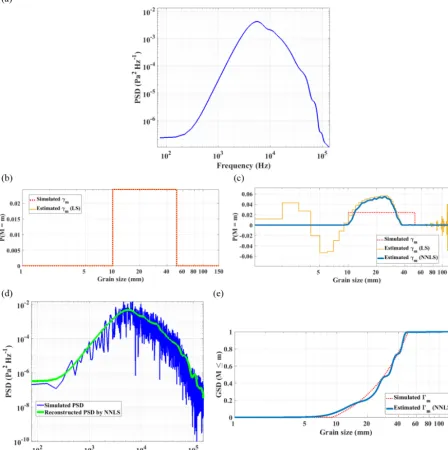
Figure 4. (a)Simulated PSD from the uniform PMFγmof sediments, 10 kg per 1 mm size class, from 10 to 50 mm, where the impact velocity isUimp=1 m s−1; the other input parameters are defined in Table 1;(b)the PMF solution obtained by the classical LS inversion, Eq. (12). The parameters used to simulate the PSD (grain size and impact velocity) shown in(a)are exactly the same as those used in modeling the dictionary1;(c)the PMF solutions obtained from the inversion of the spectrum shown in(a)using the two algebraic methods: the classical LS and the NNLS algorithm. The impact velocity used in modeling isUimp=0.1 m s−1, whereas in the simulation it isUimp=1 m s−1 (the other input parameters remain the same as in the simulation); the solutionγmis post-processed by smoothing with a Gaussian moving window of 5 mm;(d)the simulated PSD shown in(a)with added variance (see text for the noise simulation procedure);(e)the cumulative GSD obtained from the inversion of the noised spectrum by the NNNLS algorithm. The estimated solutionγ is used to reconstruct the spectrum, shown in green solid line in(d).
sphere–slab impact hasfpeak=1500 Hz, so the 200 Hz rep-resents cca. 15 % of variation between the cases.
It is worth mentioning that Uimp greatly influences the power peak, if the former is changed by 1 order of magni-tude. On the other hand, the power peak of the sphere–sphere
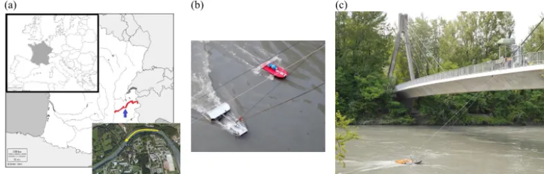
[image:7.612.75.523.75.524.2]Figure 5.Experimental setup: (a)Isère River basin geographical location (http://histgeo.ac-aix-marseille.fr) and Google Earth© picture showing the river morphology near the bridge where measurements were taken;(b)instruments used during the trials; from left to right: Toutle TR sampler and the floating river-board with hydrophone;(c)the bridge from where acoustic drifts and sediment physical samplings were realized.
a slab. This hypothesis could be supported when the riverbed is armored or paved, but may be false when the riverbed is totally mobile and when the impacts between particles of dif-ferent diameters are very common.
2.2 PSD model of the SGN generated by a mixture of sediments
In the previous section, the analytic energy spectral den-sity (ESD) was defined for the impact between a sphere and a slab. In this section, we model the power spectral density (PSD) of a sediment mixture using these analytic ESDs and the impact rate of each class of diameter, or the number of impacts per second. Assuming that particle collisions are ran-dom and independent noise sources, the model of the PSD of a mixture, denoted byP, can be expressed as a linear sum-mation of the elementary ESD, denoted byEi (Johnson and
Muir, 1969; Jonys, 1976; Thorne, 2014) weighted by the im-pact rateIi. The acoustic bedload model under discussion is
defined in the scalar form in Eq. (8) and the matrix form in Eq. (9a).
P = K
X
i=1
Ei·Ii (8)
P1 P2 .. . PNFFT
| {z }
P = E1 z}|{
E1,1
E2 z}|{
E1,2 . . .
EK z }| {
E1,K E2,1 E2,2 · · · E2,K
..
. ... . .. ...
ENFFT,1 ENFFT,2 . . . ENFFT, K
| {z }
1 · I1 I2 .. . IK
| {z }
I
⇒P =1·I (9a)
where1is the dictionary of elementary ESD of impacts be-tween spheres and slab andIis the vector of impact rates per
diameter class or, basically, a histogram. Classitakes inte-ger values, from the lowest limit, 1 mm, to the highest one,
Kmm, whereK is the largest diameter considered in mod-eling. Here, we considerKequal to 150 mm. The parameter NFFT is the number of values contained in the spectrum or the number of Fourier transform points on which the spec-trum is modeled.
The histogram I can be transformed in the probability mass functionγ by normalizing it by its sum of elements. The cumulative form ofγ will be denoted by0. Thus, one of the main assumptions is that Eq. (9a) can be written in terms of probabilitiesγ, as in Eq. (9b):
P=1·γ, (9b)
whereγi represents the probability of having a number of
impacts of particles per second for size classi.
Therefore, the random variable here isIandγis the prob-ability of impacts, and so the quantityγ(I=Ii)is a discrete probability, given that we operate on size classes of 1 mm in diameter. This probability is computed from a histogram of the number of impacts per second, so one needs to transform it into a histogram in mass of sedimentsM, to be compat-ible with the measured GSD by physical sampling. In con-sequence,γ (I=Ii)will be scaled byD3i, as in Eq. (10),
in order to obtainγm(M=mi). Finally, the grain size
dis-tribution (GSD), or the cumulative disdis-tribution form ofγm, will be0m(M≤mi), expressing the probability of sediments
finer thanDi, as defined in Eq. (11).
γm(M=mi)=κ·γ(I=Ii)·Di3, i=1, . . ., K (10) 0mj(M≤mi)=
j
X
i=1 γm
i(M=mi), j=1, . . ., K (11) whereDiis the diameter in meters andκis a constant which
2.3 Global sensitivity analysis of the spectrum generated by a mixture of sediments
This analysis was done to determine the importance of input parameters for the shape of the PSD modeled with Eq. (9b). The parameters are defined in Table 1. Global sensitivity analysis (GSA) is done to assess the impact of input pa-rameters on the model output, which in our case is the peak frequencyfpeakof spectra modeled by Eq.(9b). We use the Fourier amplitude sensitivity test (FAST) (Cukier et al., 1973) to compute the first order indices of sensitivitySi for each input parameter. The coded version of the FAST algo-rithm is presented in Cannavó (2012).
The flowchart of the GSA is presented in Fig. 3. The FAST analysis uses the typical range of parameters found in rivers, defined in the second column of Table 1. The input log-normal distributions (GSD) have median diameter values in the range from 1 to 150 mm and SDsσ from 0.01 to 10. All other input parameters needed for the model in Eq. (9b) are given in Table 1. As the output model analyzed is the peak frequency fpeak of the simulated PSD curves, the analysis does not claim to completely describe the model, but perti-nent ideas could be drawn on the model’s behavior.
The results in terms of first-order indices are presented in Table 2. The SDσ of log-normal GSD has the greatest influ-ence on the PSD shape. This is becauseσ affects the values of all percentiles of the GSD curve. The medianD50 is al-most 2 times less important thanσ. The third-greatest param-eter as a degree of influence on output is surprisingly Young’s modulus, but this is due to a very wide range of values (here
Elong=1010. . .7×1010Pa, i.e., from quartz to granite mate-rials). Such variation is not possible at the reach scale, where the sediments are of the same material. The impact velocity
Uimpcomes shortly after Young’s modulus and confirms the conclusion of the previous local analysis, that Uimp has ca. 10 % of importance in the output. Other relatively important parameters are Poisson’s ratio and the density of sediments, which means that the type of material also plays a role in the dynamics of thefpeak. The distance of measurement,r, also plays also a role in thefpeakvariation. The angle of the point of observation with respect to the impact, θ, and the prop-agation medium properties, ρandc, are considered of little influence on the values offpeak.
In conclusion, the first-order global sensitivity analysis of the peak frequency shows a comprehensive view of its dy-namics with input parameter variation. It is found that the peak frequency is mainly affected by two parameters, the dis-tribution’s SD and the median diameter, together making up
Also, the impact velocity is regarded as a minor factor of un-certainty and, because it is almost impossible to be measured for each grain size class, the 10 % uncertainty in peak fre-quency is almost unavoidable. The material properties should not be a problem with the condition that the sediments are the same. For a complete GSA, the computation of high-order sensitivity indices can be made using Sobol’s methodology (Sobol, 2001), but this type of analysis is beyond the scope of this article.
2.4 Assumptions on the proposed SGN spectrum model Modeling of single impacts requires definition of parameters typical for river environments, in Table 1. Using the global sensitivity model, it has been shown that PSD shapes are es-sentially influenced by four parameters: the shape of the GSD curve, the median diameters of the colliding particles, the impact velocities and the material. Grain sizes are estimated later using the inversion algorithm presented in Sect. 3. Con-cerning the other model parameters, as they do not affect the PSD shape, they will be fixed for the inversion process, using realistic values. These parameters are listed in the third col-umn of Table 1. The main assumptions of the SGN spectrum model are the following.
i. The geometry of the channel and of the material: the river bed is considered a massive slab and moving par-ticles are considered spherical.
ii. Sediment transport assumptions: impact velocities are assumed to be invariant with grain size. This assump-tion is supported by the relative size effects on bedload transport (Einstein, 1950; Recking, 2016; Wilcock and McArdell, 1993) referring to the mobility of finer and coarser particles.
iii. Acoustic propagation:
– as the bedload GSD is assumed to be homoge-neous everywhere in the space, the propagation ef-fects like the attenuation with distance (geometri-cal spreading models) will not impact the spectrum shape;
3 Inverse model to estimate the GSD of bedload particles
The inversion uses least square (LS) optimization methods to compute the inverse of dictionary1. NormallyK < NFFT, so 1is a non-square matrix. Moreover, the matrix1is possibly rank deficient because the spectra generated by impacts of coarser particle sizes show very similar shapes, that is, the coarser the particle, the more similar the produced sound. This is also shown in Fig. 2b, where one could observe that the points on the graph agglomerate as the grain diameters increase. In this case, the pseudo-inverse algorithm is used to solve the algebraic system of Eq. (9b). The optimization problem is defined as in Eq. (12). The least square solution to this problem is the PMF of the rate of impacts γ. The estimated PMF is further transformed into the final GSD of mass of sediments according to Eqs. (10)–(11).
ˆ
γ(I=Ii)= minimize(1+·P−γ) (12)
where 1+= 1t·1−1
·1t is the pseudo-inverse, and1t
means the transpose of the matrix1.
Eq. (12) conveys the idea of minimizing the error between the model and the measurement. This minimization opera-tion is realized in the sense of the least square optimizaopera-tion. 3.1 Numerical test of the LS method
A simulation case is proposed here to test the robustness of the LS inverse method. The simulated PMF, or grain size dis-tribution,γmis uniformly distributed between 10 and 50 mm. The uniform distribution means that 1 kg ofD=10 mm has the same probability of producing impact noise as 1 kg of
D=11 mm, and so on. To obtainγ, the simulated PMFγm is converted back to impact rates by dividing byD3,D in meters. Using an impact velocity of 1 m s−1and the rest of the input parameters defined in Table 1, the simulated PSDP is shown in Fig. 4a. Here, the dictionary1contains spectra from 1 to 150 mm and the grain size distribution has 1 mm resolution. Applying Eq. (12) on the simulated spectrum and considering exactly the same parameters in modeling and in simulation, it is found that the estimatedγm is exactly the same as the simulatedγm, as is expected; see Fig. 4b.
However, if the impact velocity used in modeling the dic-tionary is set to a value (Uimp=0.1 m s−1) which is different than the one used in simulation (Uimp=1 m s−1), then high instabilities are observed on the estimatedγm; see Fig. 4c. This is explained by the fact that there is a high similarity between the elementary spectra E, especially for the larger size classes. Thus, the matrix 1 is ill-conditioned and the problem is ill-posed. Ill-conditioning is linked to the high condition number of the normal matrix (1t.1). It is defined as the ratio between the largest and smallest eigenvalues of a matrix. A well-conditioned algebraic system requires that the normal matrix should have a condition number as close as possible to 1 (Strang, 2006). In these tests,1’s condition
number reaches huge values on the order of 1012–1020. In consequence, the similar spectra from the matrix1produce high instability in solution.
To avoid the instability in the LS solution, the non-negative least squares (NNLS) algorithm (Lawson and Hanson, 1974) is proposed to solve the LS problem. This optimization algo-rithm, Eq. (13), casts non-negative constraints on solutionγ. The non-negative factorization is widely used, for example, in various domains like image processing or chemometrics. The side-effect of using this algorithm is the strong regular-ization of solutions. The regularregular-ization aims to keep the sum of components inγ constant. The solution of the NNLS al-gorithm (see Fig. 4c) shows that the instabilities are com-pletely removed off. Besides, it is important to note that the estimated diameters are inside the simulated interval of di-ameters.
ˆ
γ(I=Ii)= minimize(1+·P−γ), γˆ ≥0 (13)
3.2 Robustness of the NNLS algorithm to PSD noise The signal processing tools in this paper refer to using the PSD as the method of spectral representation of bedload sig-nal. The use of PSD is worthwhile because the type of bed-load signal is a stationary random one. Random stationary signals are signals varying in time but whose average and SD of amplitude values over some fixed periods are constant.
A particular concern for the signal processing of random processes is the minimization of the variance on the PSD. This work makes use of the periodogram algorithm for the PSD estimation, which means the Fourier transform is ap-plied on local portions (windows) of the random signal, with an overlap of 50 %, and then the local results are averaged in narrow bandwidths (Oppenheim and Verghese, 2010). The averaging is useful because it mitigates the variance on the PSD. In this work, the quality of spectra is vital for accu-racy of estimations. The uncertainty principle tells us that the smaller the temporal window, the greater the uncertainty in locating two very close frequencies on the spectrum, so a trade must be made between the PSD variance and its spec-tral resolution. If the bedload signal is too short, the quality of spectra toward the low-frequency bands is worsened be-cause in one single bandwidth of the Fourier transform there is spectral information of impacts from multiples grain sizes. Finally, the longer the signal the better the spectral resolution and the less the variance on the PSD curve.
4 Application to real data
4.1 Isère River and experimental setup
The Isère River is a piedmont gravel river bed located in southeastern France, and it is one of the main tributaries of the Rhône River, which reaches the Mediterranean Sea. The monitoring section is located in the city of Grenoble (45◦11052.800N, 5◦46014.8800E); see Fig. 5a. In this reach, the mean slope is about 0.06 %, the area of the watershed is 5500 km2and the annual average flow rate is 180 m3s−1. At the time of experiments, 29–30 June 2016, the monitored dis-charge was on average 300 m3s−1. The measurement section has a rifle-pool morphology with riprap-protected embank-ments. Two different types of instrument were used: SGN measurements using hydrophone and direct sampling using a pressure-difference sampler, shown in Fig. 5b. All these measurements were carried out from a suspension bridge (Fig. 5c).
4.1.1 SGN measurements
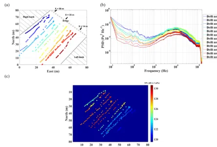
SGN measurements were made using a HTI99 hydrophone (High Tech, Inc., http://www.hightechincusa.com/) with a sensibility of−160 dB re 1 V µPa−1±3 dB from 10 Hz to 125 kHz. The hydrophone was connected to an autonomous-waterproof autonomous recorder – SDA14 (RTSYS©, http: //www.rtsys.eu). The gain of the recorder was set to 15 dB. Signals were sampled at a 312 kHz frequency with a resolu-tion of 24 bits and saved as wav files. The scope of these field experiments was to trace maps of the SGN on the local reach. The hydrophone and the recorder were attached to a free-floating river-board. The hydrophone position was about 1 m below the water surface and 1.5 m on average above the river bed. The SGN map consists in launching 12 drift measure-ments from the bridge which are located due to a GPS de-vice connected to the acoustic recorder. Each drift consists of recordings of about 30 to 40 s, or in terms of distance, between 50 and 100 m. The river-board positions during the drifts are shown in Fig. 6a. The recorded signals were pro-cessed to compute acoustic spectra. The 12 acoustic spectra recorded across the river (Fig. 6b) are inversed to estimate the bedload. The river cross section is about 60 m. Also, the 12 drift measurements are synchronized with GPS data to com-pute the SGN map in terms of sound pressure level (SPL), as is shown in Fig. 6c. The variability of SGN noise from the left to right banks can be observed from both the spectra and SPL map.
(a) the temporal waveform, in Fig. 7a; (b) the spectrogram, in Fig. 7b, as the scaled squared magnitude of short-time Fourier transform, in Pa2Hz−1; and (c) the PSD, also ex-pressed in Pa2Hz−1, computed by either averaging or medi-anizing the PSD spectrogram, in Fig. 7c. Two main sources of noise can be distinguished in the recordings: below and above 400 Hz (Fig. 7). Bedload impacts can clearly be heard in the higher frequency band, sounding like the crackling of flames. Sounds occurring below 400 Hz are non-propagating sounds as they are localized below the cutoff frequency of the river waveguide (Geay et al., 2017b; Rigby et al., 2016). They are related to turbulence-induced noise around the sen-sor and to mechanical movements of the structure sharing the hydrophone. In the Isère River experiment, the SGN sig-nal measured by drifts is almost free of hydrodynamic noise, which is proved by the typical median spectrum presented in Fig. 7c. In this study the inversion will be applied on such high signal-to-noise ratio PSD curves.
The median procedure is used to provide better smooth-ing as it filters more efficiently the unwanted low-frequency noises (Geay et al., 2017a). As in Fig. 7c, the suppression of the lower-frequency spikes can be noticed, attributed to the hydrodynamic noise, when median PSD is used instead of the average one.
4.1.3 Pressure-difference sampling
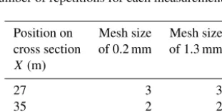
A Toutle River (TR) sampler, depicted in Fig. 5b, has been used to sample bedload particles (entrance width of 305 mm by 152 mm). There were two mesh sizes used for sampling: 0.2 and 1.3 mm. Sample durations were between 4 and 8 min. Finally, each bedload sample was dried, weighted and sieved in the laboratory. The sampled sediments were classified into six size classes:K={<0.5; 0.5–2; 2–8; 8–16; 16–32; 32– 64} mm. The TR sampler has been deployed in three cross-sectional positions (atX=27 m,X=35 m andX=44 m, marked on the bridge from the left to right river banks). The number of repetitions for each cross-sectional position is in-dicated in Table 3. Bedload fluxes (g s−1m−1) have been av-eraged for each position of the sampler. GSDs have been computed for each position and for each mesh size used. 4.2 Results
4.2.1 Direct measurements of bedload
Figure 6. (a)Positions of the floating board during drift experiments, with essential positions marked on the bridge,X={14, 35, 58} m across the river;(b)the PSD estimated from the 12 drifts, in units of Pa2Hz−1; to be noted is the change in peak frequencies: the leftmost position (Drift no. 12) has the highest frequency, meaning that the finer size fractions are transported, and the particles are getting coarser up to the right bank;(c)the measured SPL map from the 12 drifts, in units of dB re 1 µPa; the maximum values are found in the middle of the Isère River’s cross section.
Figure 7.Signal representations of the SGN recorded during hydrophone experiments on the Isère River (France):(a)temporal signal in units of Pa;(b)time–frequency representation (spectrogram), with the color code normalized with respect to power values, in Pa2Hz−1; the specific frequency bandwidth of the bedload acoustic effects and of the hydrodynamic noise agitation (extraneous sources) are indicated;(c)
[image:12.612.56.544.449.633.2]Figure 8.Measured bedload flux in three positions across the Isère River,X= {27,35,44}m and(b)measured GSD curves in these positions, using the TR sampler with two mesh sizes, 0.2 and 1.3 mm.
Figure 9. (a)Estimated GSD by the NNLS algorithm in the center of the Isère River (X=34 m), using different values of impact velocities
Uimp={0.01, 0.1, 1, 5} m s−1. Measured GSD by TR sampler (X=35 m) is represented by the yellow envelope for the two mesh sizes (see Fig. 9b for fraction sizes finer than 1 mm);(b)TheD16,D50, andD84estimated by NNLS across the Isère River compared to the regression laws of Thorne (1985, 1986b) for estimating the equivalent diameterDeq; we also indicate by arrows the range ofD50 measured by the Toutle River sampler (in positionsX= {27,35,44}m). The impact velocity used in the inversion isUimp=1 m s−1.
Table 3.Number of repetitions for each measurement.
Position on Mesh size Mesh size cross section of 0.2 mm of 1.3 mm
X(m)
27 3 3
35 2 2
44 1 2
5 times smaller, around 20 g s−1m−1. Concerning grain size distributions, most of the measurements indicate a D50 be-tween 7 and 20 mm. Notice that measurements made with the 0.2 mm mesh size towards the left bank (X=27 m) indicate a GSD toward much finer sediments (D50of about 0.3 mm) (Fig. 8b). Bedload samples closest to the left bank were
in-deed constituted of huge amounts of fine sediment mixed with vegetable debris (about 60 % of the total mass sampled). In the central and right positions, neither vegetable debris nor silts were sampled. TR sampler measurements showed grain size sorting along the river cross section, varying from silts, near the left bank, to gravel, near the right bank.
In the following, the GSD measured in the central position (X=35 m) will be considered. Its flux was indeed the largest measured, and it is considered to be the principal source of bedload noise throughout the river.
4.2.2 SGN spectra inversion
[image:13.612.101.498.284.430.2] [image:13.612.89.245.541.619.2]posi-tion of TR sampling measurements. In this posiposi-tion, it can be observed that a maximum bedload acoustic energy has been recorded. Additionally, a maximum flux of sediments was sampled in this position. The results of spectrum inversion, using a modeled dictionary1with size classes from 1 mm toK=100 mm (100 size classes), are shown in Fig. 9a. The results are compared to the GSD measured by the TR sam-pler in positionX=35 m. Four different values of the im-pact velocity Uimp are tested (from 0.01 to 5 m s−1) and it is noticed that the impact velocity Uimp between 0.01 and 0.1 m s−1 leads to a very good match between estimation and TR sampling measurements, except for the very small size classes from 1 to 5 mm. The value of impact velocity
Uimp=0.1 m s−1 will be used in the inversion of all other spectra measured across the Isère River.
Secondly, the GSD variations, represented by the per-centiles D16,D50 andD84, are estimated by the inversion of 12 drift measurements taken across the Isère River. The model uses the impact velocity of 0.1 m s−1and the rest of the parameters defined in Table 1. The estimated percentiles are compared to equivalent diametersDeq computed by re-gression laws found by Thorne (1985, 1986b) and redefined below in Eq. (14) and Eq. (15). The equivalent diameterDeq is a measure of particle size, and it is the diameter of the cir-cle with the center as the centroid mass. TheDeqis computed using fpeak and, respectively, the centroid frequencyfcentr. They are also compared to the TR sampler measurements, in the three positions across the Isère River.
fpeak= 224
D0.9 eq
, (14)
fcentr= 209
D0.88 eq
, (15)
fcentr Z
f1
Pdf = f2 Z
fcentr
Pdf, (16)
whereP is the PSD and (f1, f2) is the frequency band de-fined by a value of 10 dB below the power peak. It is ob-served that the estimated D50 by the NNLS algorithm is 10–14 mm, which is in the upper limit of the D50 mea-sured by the TR sampler (ca. 7 mm), in the middle of the river;X=35 m. On the one hand, the percentileD16almost matches the equivalent diameterDeqestimated by Thorne’s regression law fcentr(Deq), Eq. (15), which is on average 50 % below the D50 measured by the TR sampler. On the other hand, the percentileD84 is closer to the equivalent di-ameterDeqestimated by using the peak frequency regression law fpeak(Deq), Eq. (14), overestimating the measurements of the TR sampler.
5 Discussion on real data results
This work deals with the development of a novel estima-tion strategy of bedload GSD from acoustic PSD. The spec-trum inversion used the model based on sphere–slab impact, where the impacting sphere diameters range fromK=1 mm toK=100 mm. The inversion of field experiments on the Isère River have shown in Fig. 10a interesting results in con-formity with the assumptions enounced in Sect. 2.4.
The inversion considered four values of impact velocity
Uimp= {0.01;0.1;1;5}m s−1. The best fit to the measured GSD by the TR sampler is when the impact velocityUimp is between 0.01 and 0.1 m s−1, which could be possible for a large gravel bedded river like the Isère. To verify this, the apparent velocity of the bed material (see Rennie and Miller, 2004, for a definition) was measured by an aDcp at the moment of hydrophone experiments. This estimated value was at a maximum around 0.01–0.02 m s−1, which can be in accordance with the impact velocity modeling the best NNLS estimates.
The cross-sectional variation of the estimatedD16, D50 andD84 by the NNLS algorithm follows the same trend of increasing values from the left to right banks as the bed-loadD50 measured by the TR sampler (Fig. 9b). However, the cross-sectional variability of sampled diameters is higher than the estimated one. This is explained by the fact that the hydrophone has the spatial integrative characteristic (Geay et al., 2017b). The phenomenon of signal integration is typ-ical for rivers like the Isère, where high fluxes of bedload transport are concentrated only in a small portion across the section, i.e., in its center. In this case spatial homogeneity as stated in Sect. 2.4 is no longer valid. However, the powerful acoustic source makes noise all over the cross section, caus-ing the sound sources to appear ubiquitous. This may be the reason that the inversion of acoustic PSD measured in the center (X=34 m), forUimp=0.1 m s−1, still shows a good match to the sampling measurements in that position, only because of the high powerful acoustic source localized in this position.
Despite the consistent variation of the GSD across the river bed, measured by the sampler, the acoustic spectrum shapes shown in Fig. 6b are relatively stable, in the interval 5×10⁻⁴ to 5×10⁻³Pa Hz−1. This suggests that measurements by hy-drophone installed from one of the banks are not dramatically different from measurements by free floating hydrophones along the watercourse.
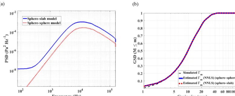
Figure 10. (a)Modeled spectra using a log-normal GSD,D=1,2, . . .,150 mm, whereD84=2D50,D50=10 mm (see medallion); typical input parameters are given in Table 1 and Uimp=1 m s−1. Concerning the sphere–sphere impact, the impactor has the same size as the impactee;(b)inversion using the NNLS algorithm by acoustic spectra shown in(a).
that the monitored spectra were slightly dependent on the hydrophone position in the lower frequency band. Another propagation effect concerns the frequency cutoff phenom-ena, due to acoustic propagation in waveguides (Geay, 2013; Geay et al., 2017b; Jensen et al., 2011; Rigby et al., 2016). In our case, the Isère River has enough large depth that the bandwidth of bedload is not being impacted. The pebble-sized particles that are up to 64 mm give SGN of dominat-ing frequencies well above 1000 Hz, whereas the channel’s depth of 2.5 m fixes the cutoff frequency to about 148 Hz, assuming a perfectly rigid bottom. Therefore, the bandwidth of bedload is far superior to the frequency cutoff in the Isère River, so there are no risks of inversion. However, SGN mon-itoring and the inversion technique for GSD determination are particularly adapted to large rivers. Generally, propaga-tion effects are frequency-dependent and higher frequency ranges are more affected by attenuation or scattering effects. A solution to the nonlinear effects of acoustic propagation would be to determine the river’s transfer function by active acoustic experiments (Rigby et al., 2016) and to construct laws of attenuation that will compensate for the loss (Wren et al., 2015).
At first sight, our comparison with Thorne (1985, 1986b)’s regression laws would be very naïve due to the nature of theories: we considered the sphere–slab impact, whereas the regression laws are from sphere–sphere impact phenomena. Therefore, the inversion is put into discussion when the river bed is no longer armored, and so, the model of impact be-tween sphere and slab is debatable. Here, we target the large gravel rivers. The dictionaries1for both impact models use an impact velocityUimp=1 m s−1, the material is granite and a GSD is simulated according to Recking’s procedure (Reck-ing, 2013), whereD84=2D50. When comparing the shapes of both simulated PSDs, shown in Fig. 10a, their respec-tive frequency peaksfpeakare nearly identical. Likewise, the
slopes of the spectra are found to be quite similar. Fig. 10b shows that the two solutions show no difference, except for a little disparity in the region of small grains. This proves that sphere–slab framework modeling of the collision between sediments and the river bed could work not only for stable conditions, but also for hydraulic events.
Another strong assumption used in modeling the PSD model of mixed impacts is that the particles are of spheri-cal shapes. It is intuitively reasoned that the particle spheric-ity, shape factor and roundness also affect the acoustics of impacts. There are multiple possible ways of reckoning the equivalent diameter of a non-spherical particle. The parti-cle’s radius may be computed with respect to the curvature of the region of contact (see Chadwick et al., 2012; Goldsmith, 2003), with respect to the particle’s mass centroid (Thorne, 1986b), which is in fact thea axis of the particle, or with respect to thebaxis of the particle (Wyss et al., 2016b). Lab-oratory tests were conducted at the GIPSA labLab-oratory, during which two pebbles of a size in the range 32–46 mm were im-pacted in a water pool along the three ellipsoid axesa,b, and
[image:15.612.106.495.68.227.2]6 Conclusion
A new strategy has been presented for data processing on hy-drophone measurements for monitoring the bedload GSD in a gravel river bed. This strategy defines a forward model and a spectrum inversion approach. Firstly, the forward model combines generated spectra from collisions between a sphere and a slab. Secondly, the inversion procedure treats the for-ward model as a linear system of equations and uses alge-braic methods of solving least square problems to obtain the GSD.
The forward model is based on a weighted sum of analyti-cal energy spectral densities modeling the physics impact be-tween a sphere and a slab. The weighting coefficients of the model represent a probability mass function which gives in the end the grain size distribution of bedload particles. The global sensitivity analysis of the PSD model of mixed im-pacts determined that the shape of the GSD has the biggest influence on the shape of the acoustic spectrum computed by Eq. (9b). Other important parameters are the median diame-ter and the impact velocity. However, the influences are from mixed interactions of parameters, and it is very hard, if not impossible, to obtain a complete analysis of the sensitivity of the analytical model of Eq. (9b).
The PSD model of mixed impacts works under the fol-lowing strong assumptions: (1) the GSD is distributed ev-erywhere in space and, in the same way, (2) the acoustic propagation is not frequency-dependent and, so, the spec-trum shape is not affected by propagation in the river, (3) the impact velocity is invariant with the grain size, and (4) the impacting particles are of a spherical shape. The in situ experimentations showed that the integrative sound from all over the reach could render the first assumption verified (or true). In the case of the Isère River, the concentration of high transport rates in the middle of the cross section permits re-liable measurements of bedload GSD by hydrophone from river banks.
The inversion method is a non-negative least square algo-rithm and it eliminates the negative solutions caused by ill-conditioned matrices. Concerning the least square approach for inversion, it is robust to noise.
The inversion of spectra from field trials on the Isère River proved that the method is highly reliable with no considera-tion of a priori informaconsidera-tion on bedform morphology of hy-drological conditions. Surrogate methods for sediment trans-port in rivers were conceived with the idea of having access to information all over the reach and real time. In contrast to geophones and the Japanese pipe, the hydrophone technique does not require particular efforts to be installed in the wa-tercourse.
Data availability. The authors provide the Matlab codes reproduc-ing the results presented in Figs. 2, 4, and 10 and Table 2. The codes are found at the following URL: https://drive.google.com/open?id= 1-eiM49Q8PW4q3acX67wlMO-NQPFXnkwi.
1 modeled dictionary of individ-ual energy spectra
Ei Energy spectral density of the
impact of the size classi, Eq. (7)
Ei,x energy of collision in a narrow
frequency bandwidth x
Pa2s Hz−1
Elong elastic modulus (Young’s mod-ulus) of rigid body
Pa ESD Energy spectral density Pa2s Hz−1
D generic notation for the grain di-ameter
mm
Deq equivalent diameter (with re-spect to the grain’s mass center)
mm
Di grain size forifrom 1 toK mm DTR grain size class measured by
Toutle River TR sampler
mm
D16, D50, D84
the 16th, 50th and 84th per-centiles of the grain size distri-bution
mm
f linear frequency Hz
fcentr centroid frequency Hz
fpeak peak frequency Hz
FAST Fourier amplitude sensitivity test
FT Fourier transform
Fs Sampling frequency Hz
F Fourier transform operator
Fimp linear complex magnitude spec-trum of the elastic impact, Eq. (5)
Pa
|Fimp|2 energy spectral density of the elastic impact, Eq. (6)
Pa2s Hz−1 GSA Global sensitivity analysis
GSD Grain size distribution
γ solution of the inversion written as a probability mass function γm solution of the inversion
writ-ten as a probability mass func-tion, computed from the mass histogram of sediments (Eq. 10) 0 solution of inversion (GSD) in
the cumulative form
0m solution of inversion (GSD) in
the cumulative form, computed fromγm(Eq. 11)
NFFT number of points for FT compu-tation
NNLS Non-negative least squares
ω Angular frequency rad s−1
P Power spectrum density of the noise from an elastic impact, Eq. (9a–b)
Pa2Hz−1
PMF Probability mass function
PSD Power spectral density Pa2Hz−1
r reference measurement distance between the sensor and the cen-ter of the impact (see Fig. 1a and b)
m
ρs density of sediment kg m−3 ρ density of water kg m−3 SGN Self-generated noise (noise
gen-erated by the transported sedi-ments in collision)
Si sensitivity indices from the
first-order global sensitivity analysis
σ the SD of a normal distribution (used in sensitivity analysis)
Td phase shift between the signals from the two objects in collision
s
t time s
τ delayed time s
t0 time variable used in the convo-lution Eq. (1)
s
θ angle of directivity acoustic sources – sensor
◦
Tc duration of Hertzian contact s Td delayed time (delayed
propaga-tion due to the geometry of par-ticles)
s
Uimp impact velocity m s−1 X position on the cross section of
the Isère River (marked on the bridge from the left to right banks)
m
Appendix B
Table B1.CoefficientsC1...6used in the analytical model of impact of Akay and Hodgson (1978).
C1 C2 C3 C4 C5 C6
αmTπ
c 2
π Tc
2 +4 ca4
4 ac3 +2Tπ
c 2
c a 4 ca
3 −2Tπ
c 2 c a 2 π Tc 3 4Tπ
c
c a
2
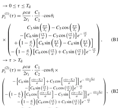
(B3). This analytical solutions model is a two-branch func-tion, depending on the duration contact Td. Thereafter, the total acoustic pressure field, during and after the impact, is obtained by subtracting the individual pressure fields. Such a resulting waveform was shown in Fig. 2a and was modeled using Eq. (B3). It is important to note that another way to compute the energy spectral density of the impact is to nu-merically compute the Fourier transform on this equation.
→0≤τ ≤Td
p(i1)(τ )=ρca 2ri
·C1 C2
·cosθi
×
C3sin
π τ Tc
−C5cos
π τ Tc
−
C6sin cτa−C5cos cτae− cτ
a +1−a
ri h
C6sin
π τ Tc
−C4sin
π τ Tc
i
−1−a ri
C6cos cτa+C5sin cτae− cτ a , (B1)
→τ > Td
p(i2)(τ )=ρca 2ri
·C1 C2
·cosθi×
−nC6sin hc(τ−T
c)
a
i +C5cos
hc(τ−T c)
a
io e−c(τ−aTc)
−C6sin cτa
−C5cos cτa
e−cτa
−1−ra
i
n C6cos
hc(τ−T c)
a
i −C5sin
hc(τ−T c)
a
io e−c(τ−aTc)
−1−ra
i
C6cos cτa
+C5sin cτa
e−cτa
, (B2)
p(τ )=p1(1)∪(2)(τ )−p2(1)∪(2)(τ−Td), (B3) where i=1 (the impacting sphere) or 2 (the mirrored sphere), both with the same radius a, τ=t−2ri−D
2c is the
delayed time,Dis the sphere’s diameter,cis the the velocity of speed,r is the reference distance,θis the angle between source and sensor (see Fig. 1b) and the constantsC1...6are
αm=
" 15 16
π Uimp2 (ζ2+ζ1)m2 √
a
#0.4
, ζ1,2=
for TP, by funding of a research grant for TG from convention no. C43R5T5030 between Électricité de France (EDF) and the Grenoble Institute of Technology, and of research grant CHORUS for Cédric Gervaise.
Edited by: Laurent Pfister
Reviewed by: two anonymous referees
References
Akay, A. and Hodgson, T. H.: Acoustic radiation fropm the elastic impact of a sphere with a slab, Appl. Acoust., 11, 285–304, 1978. Barrière, J., Krein, A., Oth, A., and Schenkluhn, R.: An ad-vanced signal processing technique for deriving grain size information of bedload transport from impact plate vibra-tion measurements, Earth Surf. Proc. Land., 40, 913–924, https://doi.org/10.1002/esp.3693, 2015.
Barton, J. S.: Passive Acoustic Monitoring of Coarse Bedload in Mountain Streams, The Pennsylvania State University, College State, USA„ 2006.
Bedeus, K. and Ivicsis, L.: Observation of the noise of bed load, Int. Assoc. Hydrol. Sci., 19–31, 1963.
Belleudy, P., Valette, A., and Graff, B.: Passive hydrophone moni-toring of bedload in river beds: first trials of signal spectral anal-yses, USGS, Scientific Investigations Report, 5091, 67–84, Vir-ginia, USA, 2010.
Bogen, J. I. M. and Møen, K.: Bed load measurements with a new passive ultrasonic sensor, Erosion and Sediment Transport Mea-surement: Technological and Methodological Advances, Interna-tional Association of Hydrological Sciences, Oslo, 19–21, 2001. Bunte, K. and Abt, S.: Sampling Surface and Subsurface Particle-Size Distributions in Wadable Gravel- and Cobble-Bed Streams for Analyses in Sediment Transport, Hydraulics, and Streambed Monitoring, Gen. Tech. Rep. RMRS-GTR-74., Forest Service, Rocky Mountain Research Station, Fort Collins, Colorado, U.S. Department of Agriculture, 2001.
Bunte, K., Swingle, K. W., and Abt, S. R.: Necessity and Diffi-culties of Field Calibrating Signals from Surrogate Techniques in Gravel-Bed Streams: Possibilities for Bedload Trap Sam-plers, US Geol. Surv. Sci. Investig. Rep. 2010-5091, Bedload-Surrogate Monitoring Technologies, US Geol. Surv. Sci. Invest. Rep, 5091, 107–129, Virginia, USA, 2010.
Cannavó, F.: Sensitivity analysis for volcanic source modeling qual-ity assessment and model selection, Comput. Geosci., 44, 52–59, https://doi.org/10.1016/j.cageo.2012.03.008, 2012.
Chadwick, J. N., Zheng, C., and James, D. L.: Precomputed accel-eration noise for improved rigid-body sound, ACM T. Graphic., 31, 1–9, https://doi.org/10.1145/2185520.2335454, 2012. Cukier, R. I., Fortuin, C. M., Shuler, K. E., Petschek, A. G., and
Schaibly, J. H.: A Study of the Sensitivity of Coupled Reaction
in open channel flows, Soil Conserv. Serv., 1026, 1–31, 1950. European Commission: European Common Implementation
Strat-egy for the Water Framework Directive (2000/60/EC), Water Di-rectors under Swedish Presidency, Directive, 428, May, 2001. Geay, T.: Mesure acoustique passive du transport par charriage dans
les rivières [Passive Acoustic measurement of bedload transport in rivers], Université Joseph Fourier, Grenoble, 2013.
Geay, T., Belleudy, P., Gervaise, C., Habersack, H., Aigner, J., Kreisler, A., Seitz, H., and Laronne, J.: Passive acoustic monitor-ing of bedload in large gravel bed rivers, J. Geophys. Res.-Earth, 122, 528–545, https://doi.org/10.1002/2016JF004112, 2017a. Geay, T., Belleudy, P., Laronne, J. B., Camenen, B.,
Ger-vaise, C., and Development, E.: Spectral variations of under-water river sounds 1, Earth Surf. Proc. Land., 42, 2447–2456, https://doi.org/10.1002/esp.4208, 2017b.
Gimbert, F., Tsai, V. C., and Lamb, M. P.: A physical model for seis-mic noise generation by turbulent flow in rivers, J. Geophys. Res. Earth, 119, 2209–2238, https://doi.org/10.1002/2014JF003201, 2014.
Goldsmith, W.: Impact, Dover Publications, Inc., Mineola, NY, USA, 2003.
Gray, J. R., Laronne, J. B., and Marr, J. D. G.: Bedload-surrogate monitoring technologies, US Geol. Surv. Sci. Investig. Rep., 5091, 1–37, available at: https://pubs.usgs.gov/sir/2010/5091/ (last access: 10 January 2013), 2010.
Heimann, F. U. M., Rickenmann, D., Turowski, J. M., and Kirch-ner, J. W.: sedFlow – a tool for simulating fractional bedload transport and longitudinal profile evolution in mountain streams, Earth Surf. Dynam., 3, 15–34, https://doi.org/10.5194/esurf-3-15-2015, 2015.
Hertz, H.: Über die Berührung fester elastischer Körper (On the vi-bration of solid elastic bodies), J. Reine Angew. Math., 92, 156– 171, 1882.
Hubbell, D. W.: Apparatus and Techniques for Measuring Bedload, US Geol. Surv. Water-Supply Pap., US Govt. Print. Off., Wash-ington, USA, 1748, 74, 1964.
Hunter, S. C.: Energy absorbed by elastic waves during impacts, J. Mech. Phys. Solids, 5, 162–171, 1957.
Jensen, F. B., Kuperman, W. A., Porter, M. B., and Schmidt, H.: Computational Oceanic Acoustics, Springer-Verlag, New York, 2011.
Johnson, P. and Muir, T. C.: Acoustic detection of sediment movement, J. Hydraul. Res., 7, 519–540, https://doi.org/10.1080/00221686909500283, 1969.
Jonys, C. K.: Acoustic measurement of sediment transport, Sci. Ser., 66, 1–64, 1976.
Kirchhoff, G. R.: Vorlesungen uber Matematische Physik”, Vol. 1, “Mechanik”, Dritte Auflage, Druck und Verlag von G. B. Teub-ner, Leipzig, 1, 316–320, 1883.
Krein, A., Klinck, H., Eiden, M., Symader, W., Bierl, R., Hoff-mann, L., and Pfister, L.: Investigating the transport dynam-ics and the properties of bedload material with a hydro-acoustic measuring system, Earth Surf. Proc. Land, 33, 152–163, https://doi.org/10.1002/esp.1576, 2008.
Krein, A., Schenkluhn, R., Kurtenbach, A., Bierl, R., and Barrière, J.: Listen to the sound of moving sediment in a small gravel-bed river, Int. J. Sediment Res., 31, 271–278, https://doi.org/10.1016/j.ijsrc.2016.04.003, 2014.
Kuhnle, R. A.: Fluvial transport of sand and gravel mixtures with bimodal size distributions, Sediment. Geol., 85, 17–24, https://doi.org/10.1016/0037-0738(93)90072-D, 1993.
Lawson, C. L. and Hanson, R. J.: Solving Least-Squares Problems, Englewood Cliffs, NJ: Prentice Hall, 23, 161 pp., 1974. Mao, L., Carrillo, R., Escauriaza, C., and Iroume, A.: Flume
and field-based calibration of surrogate sensors for mon-itoring bedload transport, Geomorphology, 253, 10–21, https://doi.org/10.1016/j.geomorph.2015.10.002, 2016.
Mizuyama, T., Oda, A., Laronne, J. B., Nonaka, M., and Mat-suoka, M.: Laboratory tests of a japanese pipe geophone for continuous acoustic monitoring of coarse bedload, Bedload-Surrogate Monit. Technol., USGS, Scientific Investigations Re-port, 5091, 319–335, 2010.
Muste, M., Baranya, S., Tsubaki, R., Kim, D., Ho, H., Tsai, H., and Law, D.: Acoustic mapping velocimetry, Water Resour. Res., 52, 4132–4150, https://doi.org/10.1002/2015WR018354, 2016. Oppenheim, A. V and Verghese, G. C.: Signals, Systems and
Inference – Class notes for 6.011: Introduction to Com-munication, Control and Signal Processing Spring 2010, Cl. notes 6.011 Introd. to Commun. Control Signal Pro-cess. – Massachusetts Inst. Technol., available at: http: //scholar.google.com/scholar?hl=en&btnG=Search&q=intitle: Signals,+systems+and+inference#8, 2010.
Papanicolaou, A. N. (Thanos), Elkaheem, M., and Knapp, D.: Evaluation of a gravel transport sensor for bed load mea-surements in natural flows, Int. J. Sediment Res., 24, 1–15, https://doi.org/10.1016/S1001-6279(09)60012-3, 2009. Parker, G.: Surface-based bedload transport relation
for gravel rivers, J. Hydraul. Res., 28, 417–436, https://doi.org/10.1080/00221689009499058, 1990.
Parker, G.: Chapter 3: Transport of gravel and sediment mixtures, ASCE, 54, 1–162, 2002.
Recking, A.: An analysis of nonlinearity effects on bed load transport prediction, J. Geophys. Res.-Earth, 118, 1264–1281, https://doi.org/10.1002/jgrf.20090, 2013.
Recking, A.: A generalized thresholdmodel for computing bed load grain size distribution, Water Resour. Res., 52, 1–15, https://doi.org/10.1029/2008WR006912, 2016.
Rennie, C. D. and Millar, R. G.: Measurement of the spa-tial distribution of fluvial bedload transport velocity in both sand and gravel, Earth Surf. Proc. Land., 29, 1173–1193, https://doi.org/10.1002/esp.1074, 2004.
Rickenmann, D., Turowski, J. M., Fritschi, B., Wyss, C., Laronne, J., Barzilai, R., Reid, I., Kreisler, A., Aigner, J., Seitz, H., and Habersack, H.: Bedload transport measurements with impact plate geophones: comparison of sensor calibration in different gravel-bed streams, Earth Surf. Proc. Land., 39, 928– 942, https://doi.org/10.1002/esp.3499, 2014.
Rigby, J. R., Wren, D., and Murray, N.: Acoustic Signal Propagation and Measurement in Natural Stream Channels for Application to Surrogate Bed Load Measurements, Halfmoon Creek, Colorado, 1566–1570, 2016.
Roth, D. L., Brodsky, E. E., Finnegan, N. J., Rickenmann, D., Tur-owski, J. M., and Badoux, A.: Bed load sediment transport in-ferred from seismic signals near a river, J. Geophys. Res.-Earth, 121, 725–747, https://doi.org/10.1002/2015JF003782, 2016. Sobol, I. M.: Global sensitivity indices for nonlinear
math-ematical models and their Monte Carlo estimates, Math. Comput. Simulat., 55, 271–280, https://doi.org/10.1016/S0378-4754(00)00270-6, 2001.
Strang, G.: Linear Algebra and Its Applications, Thomson Brooks-Cole Publishing, Pacific Grove CA, USA, 487 pp., 2006. Thorne, P. D.: The measurement of acoustic noise generated by
moving artificial sediments, J. Acoust. Soc. Am., 78, 1013–1023, 1985.
Thorne, P. D.: An intercomparison between visual and acoustic detection of seabed gravel movement, Mar. Geol., 72, 11–31, https://doi.org/10.1016/0025-3227(86)90096-4, 1986a.
Thorne, P. D.: Laboratory and marine measurements on the acoustic detection of sediment transport, J. Acoust. Soc. Am., 80, 899– 910, https://doi.org/10.1121/1.393913, 1986b.
Thorne, P. D.: An overview of underwater sound generated by in-terparticle collisions and its application to the measurements of coarse sediment bedload transport, Earth Surf. Dynam., 2, 531– 543, https://doi.org/10.5194/esurf-2-531-2014, 2014.
Thorne, P. D. and Foden, D.: Generation of underwater sound by colliding spheres, J. Acoust. Soc. Am., 84, 2144–2152, https://doi.org/10.1121/1.397060, 1988.
Tsai, V. C., Minchew, B., Lamb, M. P., and Ampuero, J.-P.: A physical model for seismic noise generation from sediment transport in rivers, Geophys. Res. Lett., 39, https://doi.org/10.1029/2011GL050255, 2012.
Turowski, J. M., Badoux, A., and Rickenmann, D.: Start and end of bedload transport in gravel-bed streams, Geophys. Res. Lett., 38, 1–5, https://doi.org/10.1029/2010GL046558, 2011.
Wilcock, P. R. and Kenworthy, S. T.: A two-fraction model for the transport of sand/gravel mixtures, Water Resour. Res., 38, 1–12, https://doi.org/10.1029/2001WR000684, 2002.
Wilcock, P. R. and McArdell, B. W.: Surface-based fractional trans-port rates: mobilization thresholds and partial transtrans-port of a sand-gravel sediment, Water Resour. Res., 29, 1297–1312, 1993. Wilcock, P., Pitlick, J., and Cui, Y.: Sediment Transport Primer:
Es-timating Bed-Material Transport in Gravel-Bed Rivers, Rocky Mountain Research Station, USDA Forest Service, RMRS-GTR-226, 2009.
Wren, D. G., Goodwiller, B. T., Rigby, J. R., Carpenter, W. O., Kuhnle, R. A., and Chambers, J. P.: Sediment-Generated Noise (SGN): laboratory determination of measurement volume, Proc. 3rd Jt. Fed. Interag. Conf., 10th Fed. Interag. Sediment. Conf. 5th Fed. Interag. Hydrol. Model. Conf. 19–23 Apr 2015, Reno, Nevada, D, 408–413, 2015.