Disinformative data in large scale hydrological modelling

Hydrol. Earth Syst. Sci., 17, 2845–2857, 2013 www.hydrol-earth-syst-sci.net/17/2845/2013/ doi:10.5194/hess-17-2845-2013

© Author(s) 2013. CC Attribution 3.0 License.

EGU Journal Logos (RGB)

Advances in

Geosciences

Open Access

Natural Hazards

and Earth System

Sciences

Annales

Geophysicae

Nonlinear Processes

in Geophysics

Atmospheric

Chemistry

and Physics

Atmospheric

Chemistry

and Physics

Atmospheric

Measurement

Techniques

Atmospheric

Measurement

Techniques

Biogeosciences

Open Access Open Access

Biogeosciences

Discussions

Climate

of the Past

Open Access Open Access

Climate

of the Past

Discussions

Earth System

Dynamics

Open Access Open Access

Earth System

Dynamics

Geoscientific

Instrumentation

Methods and

Data Systems

Open Access

_{Geoscientific}

Instrumentation

Methods and

Data Systems

Geoscientific

Model Development

Open Access Open Access

Geoscientific

Model Development

Hydrology and

Earth System

Sciences

Hydrology and

Earth System

Sciences

Ocean Science

Open Access Open Access

Ocean Science

Discussions

Solid Earth

Open Access Open Access

Solid Earth

Discussions

The Cryosphere

Open Access Open Access

The Cryosphere

Discussions

Natural Hazards

and Earth System

Sciences

Open Access

Discussions

Disinformative data in large-scale hydrological modelling

A. Kauffeldt1, S. Halldin1, A. Rodhe1, C.-Y. Xu1,2, and I. K. Westerberg1,3,4 1_{Department of Earth Sciences, Uppsala University, Uppsala, Sweden}

2_{Department of Geosciences, University of Oslo, Oslo, Norway} 3_{IVL Swedish Environmental Research Institute, Stockholm, Sweden} 4_{Department of Civil Engineering, University of Bristol, Bristol, UK}

Correspondence to: A. Kauffeldt ([email protected])

Received: 14 December 2012 – Published in Hydrol. Earth Syst. Sci. Discuss.: 14 January 2013 Revised: 1 May 2013 – Accepted: 2 June 2013 – Published: 22 July 2013

Abstract. Large-scale hydrological modelling has become

an important tool for the study of global and regional wa-ter resources, climate impacts, and wawa-ter-resources manage-ment. However, modelling efforts over large spatial domains are fraught with problems of data scarcity, uncertainties and inconsistencies between model forcing and evaluation data. Model-independent methods to screen and analyse data for such problems are needed. This study aimed at identifying data inconsistencies in global datasets using a pre-modelling analysis, inconsistencies that can be disinformative for sub-sequent modelling. The consistency between (i) basin ar-eas for different hydrographic datasets, and (ii) between cli-mate data (precipitation and potential evaporation) and dis-charge data, was examined in terms of how well basin ar-eas were represented in the flow networks and the possibility of water-balance closure. It was found that (i) most basins could be well represented in both gridded basin delineations and polygon-based ones, but some basins exhibited large area discrepancies between flow-network datasets and archived basin areas, (ii) basins exhibiting too-high runoff coefficients were abundant in areas where precipitation data were likely affected by snow undercatch, and (iii) the occurrence of basins exhibiting losses exceeding the potential-evaporation limit was strongly dependent on the potential-evaporation data, both in terms of numbers and geographical distribution. Some inconsistencies may be resolved by considering sub-grid variability in climate data, surface-dependent potential-evaporation estimates, etc., but further studies are needed to determine the reasons for the inconsistencies found. Our results emphasise the need for pre-modelling data analysis to identify dataset inconsistencies as an important first step in any large-scale study. Applying data-screening methods

before modelling should also increase our chances to draw robust conclusions from subsequent model simulations.

1 Introduction

Large-scale hydrological modelling has become a focal point in hydrological research in recent years and is of fundamen-tal importance for understanding continenfundamen-tal and global wa-ter balances, impacts of climate and land-use changes, and for water-resources management (e.g. Jung et al., 2012; Li et al., 2012; Mulligan, 2012; Werth and G¨untner, 2010). How-ever, hydrological modelling and analysis of large spatial do-mains is severely constrained by data availability and qual-ity (Arnell, 1999a; Decharme and Douville, 2006; D¨oll and Siebert, 2002; Fekete et al., 2004; G¨untner, 2008; Hunger and D¨oll, 2008; Peel et al., 2010; Wid´en-Nilsson et al., 2009). In addition, the modellers’ knowledge of the quality and limi-tations of large-scale datasets is often inevitably inadequate, which restricts the possibility to distinguish informative from disinformative data.

Beven et al. (2011) use a master recession curve to identify rainfall-runoff events with inconsistent runoff coefficients for a British catchment, i.e. events where the water balance be-tween precipitation input and discharge output is not satis-fied, periods that they show are “disinformative” in model evaluation. Westerberg et al. (2011) develop a model evalua-tion criterion that can be expected to be more robust to some types of moderate disinformation and analyse the effect of disinformative data periods on model inference in a posterior analysis. Kuczera (1996) shows that rating curve errors can “very substantially, indeed massively” corrupt design-flood estimation. When accounting for precipitation errors in cali-bration of a watershed model, Vrugt et al. (2008) found that the posterior distribution of the parameters and the model predictive uncertainty were significantly affected. Beven and Westerberg (2011) discuss the difficulties in analysing in-formation/disinformation content in hydrological data given multiple sources of epistemic data errors and their interac-tion with model-structural errors. They highlight the impor-tance of isolating disinformative data periods independent of a model and then excluding them from model calibration and evaluation. Model-independent methods to identify disinfor-mative data and to investigate the effect of different types of disinformation on model inference need to be further devel-oped. These research questions are particularly relevant for global hydrological models (GHMs) that are severely data constrained and where model fit is sometimes only anecdo-tally described. Substantial correction and tuning factors are reported for GHMs in order to achieve acceptable fit to ob-served discharge data (e.g. Fekete et al., 1999; Hunger and D¨oll, 2008; Palmer et al., 2008). At the large scale it is im-possible for the modeller to have the same detailed knowl-edge of the quality and limitations of the modelling datasets as on the local catchment scale. This effectively restricts the possibility to distinguish informative data from disinforma-tive ones, and calls for new types of analysis methods.

GHMs are commonly evaluated against discharge since it represents an aggregated hydrological response of a basin. Selection of basins for calibration/evaluation purposes has previously been done mainly on the grounds of basin size and record-length thresholds (e.g. D¨oll et al., 2003; Fekete et al., 1999).

Many GHMs operate at a spatial resolution of 0.5◦×0.5◦ longitude and latitude, which corresponds to a cell area of approximately 3100 km2at the Equator (e.g. Arnell, 1999a; D¨oll et al., 2003; V¨or¨osmarty et al., 1989; Wid´en-Nilsson et al., 2007, 2009), or even at a coarser resolution (e.g. Hanasaki et al., 2008) and can therefore not be expected to represent small basins very well. The low resolution of GHMs leads to a trade-off between using discharge stations with small basin areas for spatial coverage and excluding them since their representation in coarse flow networks is restricted. Previous global studies have set minimum area thresholds to 9000 (D¨oll et al., 2003; Kaspar, 2004) and 10 000 km2(Fekete et al., 1999, 2002), and further reduced

the number of basins based on interstation-area (i.e. area be-tween river gauges) thresholds of 20 000 and 10 000 km2, re-spectively. Hanasaki et al. (2008) use an area threshold of 200 000 km2, but their model works at a lower spatial res-olution (1◦×1◦ longitude and latitude). Yet other studies have limited the evaluation to only a few major river basins (e.g. Nijssen et al., 2001).

Recent development of high-resolution hydrographic datasets such as HydroSHEDS (Lehner et al., 2008) offers the possibility to use high-resolution topographic data in global modelling, e.g. for runoff routing (Gong et al., 2011) and for representation of sub-grid-scale topography in flood-plain inundation modelling (Yamazaki et al., 2009, 2011). This has also led to development of new up-scaled datasets and high-resolution basin delineations. This sparks the ques-tion whether smaller basins than used in previous studies can be utilised for calibration/evaluation of GHMs and what re-strictions to basin size are imposed by input data, since pre-cipitation for longer periods than the last decades is com-monly only available at 0.5◦×0.5◦resolution.

The global hydrological-modelling community lacks a methodology to evaluate forcing and calibration data inde-pendent of a specific model, which hampers comparisons of results from different models. In order to be right for the right reasons, a global modelling effort should start with an evaluation of data quality and, especially, possible in-consistencies between datasets. This paper presents a basic pre-modelling analysis of large-scale hydrological datasets. The overall goal of the paper was to address the problem of physically inconsistent and therefore disinformative data in large-scale hydrological modelling and to show the impor-tance of a pre-modelling data analysis. The study was per-formed in two steps. The first step was to evaluate how well basin areas were represented in three gridded (0.5◦×0.5◦) hydrography datasets and one high-resolution GIS dataset (derived from 15 arc-second topography) for basins as small as 5000 km2. The second was to analyse and identify in-consistencies between GHM forcing and evaluation data by comparing four precipitation datasets and three potential-evaporation datasets (all gridded at 0.5◦resolution) with ob-served discharge.

2 Data

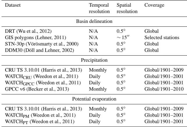
Table 1. Summary of global datasets used in the study.

Dataset Temporal Spatial Coverage

resolution resolution

Basin delineation

DRT (Wu et al., 2012) N/A 0.5◦ Global

GIS polygons (Lehner, 2011) N/A ∼1500 Selected stations

STN-30p (V¨or¨osmarty et al., 2000) N/A 0.5◦ Global

DDM30 (D¨oll and Lehner, 2002) N/A 0.5◦ Global

Precipitation

CRU TS 3.10.01 (Harris et al., 2013) Monthly 0.5◦ Global/1901–2009

WATCH_CRU(Weedon et al., 2011) Daily 0.5◦ Global/1901–2001

WATCHGPCC(Weedon et al., 2011) Daily 0.5◦ Global/1901–2001

GPCC v6 (Becker et al., 2013) Monthly 0.5◦ Global/1901–2010

Potential evaporation

CRU TS 3.10.01 (Harris et al., 2013) Monthly 0.5◦ Global/1901–2009

WATCHPM(Weedon et al., 2011) Daily 0.5◦ Global/1901–2001

WATCHPT(Weedon et al., 2011) Daily 0.5◦ Global/1901–2001

(above 60◦N) and HydroSHEDS (Lehner et al., 2008) for the rest of the land surface. Digital elevation data from Hy-droSHEDS (1500resolution) were used for visualisation pur-poses. All gridded basin-delineation datasets covered the whole globe, whereas the polygon dataset only covered se-lected basins (Table 1).

Discharge data were obtained from GRDC in June 2011, at which time the archive held records for 7763 discharge stations worldwide. Record lengths varied considerably be-tween stations. Only monthly data calculated by GRDC from daily records were used because these data contain correc-tions performed by the providers, such as changes in rating curves, etc. (T. de Couet, GRDC, personal communication, July 2011).

Precipitation datasets included in the study were the Cli-mate Research Unit’s freely available CRU TS 3.10.01 cli-mate data (Harris et al., 2013; see Mitchell and Jones, 2005, for version 2.1), GPCC Full Data Reanalysis version 6 (data provided by NOAA/OAR/ESRL PSD, Boulder, Colorado, USA, from www.esrl.noaa.gov/psd/) and both the CRU and the GPCC bias-corrected WATCH forcing data, from here on called WATCHCRUand WATCHGPCC(Weedon et al., 2011).

The CRU TS 2.1 precipitation dataset is based on ground observations from several sources and each station has been subjected to an iterative homogenisation procedure to de-tect and correct discontinuities (e.g. caused by changes in instrumentation). Station records have then been converted to relative anomalies compared to the 1961–1990 standard period. The anomalies have been spatially interpolated to a 0.5◦ latitude-longitude grid before being combined with 1961–1990 normals from New et al. (1999) to a grid of ab-solute values (Mitchell and Jones, 2005). Gauge undercatch has not been explicitly corrected, but the 1961–1990 normals

were based on both corrected and uncorrected stations, which means some areas are implicitly corrected (Mitchell and Jones, 2005; New et al., 1999). The major difference between the CRU TS 3.10.01 precipitation dataset and the version de-scribed in Mitchell and Jones (2005), apart from longer cov-erage (up to the end of 2009 compared to 2002) and inclusion of new station data, is that no new homogenisation has been performed on CRU TS 3.10.01 (BADC, 2013).

The GPCC precipitation dataset is, just as CRU, a rain-gauge-based dataset derived by spatially interpolat-ing anomalies from quality-controlled station records and combining them with a background climatology to obtain monthly gridded precipitation. However, the number of sta-tions on which the GPCC product is based (∼67 200) by far exceeds the CRU collection (∼11 800). The GPCC precip-itation dataset does not include corrections for gauge mea-surement errors (Becker et al., 2013).

As opposed to the CRU and GPCC precipitation datasets, the WATCH precipitation data are not based on observed data, but on the European Centre for Medium-Range Fore-casts (ECMWF) 40 yr reanalysis, ERA-40 (Uppala et al., 2005). However, two earlier versions of the CRU (ver-sion 2.1) and GPCC (ver(ver-sion 4) data products have been used to correct ERA-40 precipitation for known biases (e.g. Hagemann et al., 2005). Bias correction has been done in two steps: (i) the number of wet days has been adjusted to match the observations in CRU if the number of wet days in ERA-40 exceeded the number of wet days in CRU, and (ii) the monthly precipitation totals have been adjusted to match either CRU or GPCC, thereby creating two different precipitation datasets (WATCHCRU and WATCHGPCC).

0.96

0.86 0.84

0.73 0.55

0.29

0.28 0.18

0.1

0.12

0.02 0.02

0.01 0.01

0.01 DRT Basin Outline

Polygon Basin Outline

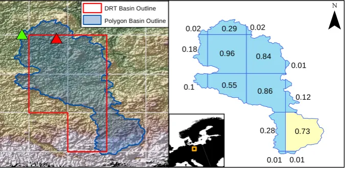
Fig. 1. Example of treatment of gridded climate data for the polygon basin delineations. Basin outline based on DRT and GIS-polygon

data for Berlin M¨uhlendamm UP discharge station on the Spree River (9707 km2) overlaid on 0.5◦climate data grid (left panel). Basin

intersections with the climate grid cells labelled with the fraction of the intersecting grid area (right). For each climate grid cell, only the intersecting fraction contributes to the basin average: e.g. for the yellow polygon 73 % of the precipitation falling in the climate grid cell is assumed to fall within the basin. The red triangle indicates the location of the gauge according to the GRDC archive and the green triangle the location after corrections made in the generation of the GIS-polygon dataset.

catch quotients for liquid and solid precipitation from Adam and Lettenmaier (2003). Since the ERA-40 reanalysis prod-uct only covers 1958–2001, reordered ERA-40 data have been used for the period 1901–1957 (Weedon et al., 2011).

Potential evaporation is available from the CRU and the WATCH datasets. Both the CRU and the WATCH datasets provide estimates based on the Food and Agricultural Orga-nization (FAO) reference-crop-evaporation equation (Allen et al., 1994). In this version of the Penman–Monteith equa-tion (Monteith, 1965), a hypothetical well-watered refer-ence crop is defined with a height of 0.12 m, an albedo of 0.23, a surface resistance of 70 s m−1 and an aerody-namic resistance based on the crop height and wind speed. The CRU estimates were calculated from monthly gridded values of average/minimum/maximum temperatures, vapour pressure and cloud cover, and fixed monthly wind speeds for the standard period 1961–1990 (Harris et al., 2013). The WATCH FAO Penman–Monteith (WATCHPM) dataset

is based on 3-hourly bias-corrected ERA-40 data (Weedon et al., 2011). The WATCH dataset also provides estimates based on the Priestley–Taylor equation (Priestley and Taylor, 1972) assuming an albedo of 0.23 and theαfactor set to 1.26 (Weedon et al., 2011).

3 Method

3.1 Climate and discharge data

Climate data were attributed to grid cells defined as land in the basin delineations, but not covered by the climate datasets, in an iterative manner to an average of the clos-est surrounding cells covered by the climate datasets until all

land areas were covered. For the GIS-polygon dataset, the in-tersections with the half-degree climate-data grid cells were used to calculate the fraction of precipitation and potential evaporation of each cell contributing to the basin (Fig. 1). Sub-grid variability was not taken into account, i.e. precipi-tation and potential evaporation were assumed to be evenly distributed over each grid cell.

Only data within the common period of the climate datasets (1901–2001) were used in the analysis, and peri-ods for individual basins varied depending on the discharge-data records. The quality control of discharge discharge-data in this study was limited to an elimination of clearly erroneous data (i.e. wrongly set nulls such as 999 instead of the correct miss-ing data value of−999). When these appeared in the daily data, the monthly data were also excluded.

3.2 Hydrography representation of basin areas

if the flow-accumulation area of any of the closest eight sur-rounding cells better corresponded to the basin area reported by GRDC. And thirdly, all stations exhibiting a relative area difference,εA, of more than 10% were manually inspected

and re-assigned if possible. The relative area difference was calculated according to Eq. (1). This measure was adopted since it has been used previously (D¨oll and Lehner, 2002; Fekete et al., 1999) but under the name “symmetric error”. It was termed relative area difference in this study to clarify that no assumption was made about the error distribution.

εA =

AAcc−AGRDC

max(AAcc, AGRDC)

·100 %, (1)

AAccis the flow-accumulation area of the assigned cell and

AGRDCis the GRDC basin area. Positive (negative) relative

area differences mean that calculated basin areas are larger (smaller) than the ones reported to GRDC. The inspection was done in Google Earth by using online map resources and superimposing the flow network on a 1:10 000 000 river net-work (freely available from www.naturalearthdata.com; ac-cessed on 17 October 2011).

We calculated cell areas for all the gridded hydrographic datasets as quadrangles based on the World Geodetic Sys-tem 1984 ellipsoid. The relative area differences for all hy-drographic datasets were calculated and used to evaluate how well the different datasets represented basin areas in compar-ison to the areas reported in the GRDC database.

3.3 Evaluation of consistency between model forcing and evaluation data

Similarly to Beven et al. (2011), the basic method used in this study was to identify disinformative data as those that violate the conservation equation, i.e. the water balance. In contrast to their event-based approach we analysed the long-term wa-ter balance and also analysed data for transgressions of the potential-evaporation limit, similarly to Peel et al. (2010). The change in basin storage can safely be ignored for suf-ficiently long time periods, except for special cases such as melting glaciers. The water-balance equation can then be simplified to

P =EA+R, (2)

where P is precipitation, EA actual evaporation and R

runoff. For natural basins, runoff should not exceed the pre-cipitation input to the system. Actual evaporation equals the difference between precipitation and runoff and should not exceed potential evaporation (EP). These were the

funda-mental assumptions on which the consistency checks be-tween the forcing data (precipitation and potential evapora-tion) and the evaluation data (discharge) were based.

All datasets are affected by different types of uncertainties. Estimating them can be difficult because of lack of knowl-edge about their nature and magnitude, both temporally

and spatially. There is a growing literature on quantifica-tion of uncertainties connected to hydrological modelling, reviewed by McMillan et al. (2012), concerning magni-tudes of observational uncertainties of some key hydrolog-ical variables. In the present study, a relative uncertainty of ±10 % was assumed for long-term discharge (resulting in a low, a high and a best (i.e. the original data) estimate for each time series). Climate data were used as given in their original sources, which means that potential evapora-tion refers to FAO Penman–Monteith reference-crop esti-mates for WATCHPM and CRU and to Priestley–Taylor

es-timates for WATCHPT and, hence that land cover is not

ex-plicitly taken into account.

The runoff coefficient (RC), i.e. the quotient of runoff to precipitation, is a measure of how precipitation is partitioned into runoff and evaporation. RCs are often calculated on an event basis and for specific surfaces, but can also be de-termined as a long-term response characteristic for a basin. Long-term RCs were calculated for low, high and best es-timated discharge values, resulting in a high, a low, and a best-estimate RC value for each basin. Hence, the first test of consistency between datasets, that runoff should not exceed precipitation input, stated that RCs should not be higher than one. In reality, a long-term basin RC even close to unity is implausible if the basin definition is correct, since it means that even over several years hardly any flux to the atmo-sphere would occur. Even in very cold systems losses occur through sublimation from intercepted snow and from snow on the ground (e.g. Strasser et al., 2008). Unity was used as a conservative threshold in this study to avoid classify-ing datasets as inconsistent based on arbitrary RC thresholds. When based on low estimates of RC values, this threshold could be considered very conservative.

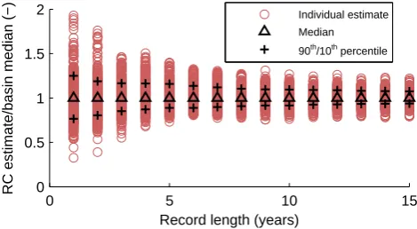
In order to investigate when time periods were “suffi-ciently” long to determine long-term runoff coefficients, an initial analysis was performed of the variation of RCs with regards to record length. A subset (n= 37) was selected of the co-registered GRDC stations with complete data through-out the common period (January 1901–December 2001). For each record length (1 to 15 yr of consecutive data), each dis-charge record was randomly re-sampled 20 times (overlaps occurred) and the runoff coefficient for each sample was cal-culated. For each basin and sample length, the individual RC estimates were divided by the median RC and plotted for all 37 basins (Fig. 2). It was assumed from the spread in the scat-ter plot that 10 yr of data sufficed to estimate the long-scat-term runoff coefficients.

0 5 10 15 0

0.5 1 1.5 2

RC estimate/basin median (−)

Record length (years)

Individual estimate Median

90th_/10th _percentile

Fig. 2. Variation of runoff-coefficient estimates as a function of

record length summarised for 37 basins with long data records. Esti-mates are standardised by division with the basin median for a given record length.

4 Results

4.1 Hydrography representation of basin area

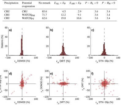
Of the 7763 stations available in the GRDC data archive, 245 stations were excluded from the study because of in-sufficient metadata records, i.e. missing coordinates or basin areas. The remaining 7518 stations with sufficient metadata were registered in the DRT flow network following only the two automatic steps at first. Many stations in the database represented basins smaller than a 0.5◦ cell and clear sys-tematic errors because of overestimated areas for these small basins were noticed in this initial stage (Fig. 3). Since man-ual checking of station locations is very time consuming, the study was limited to basins larger than 5000 km2. This threshold is considerably smaller than those of previous stud-ies but it still meant that most small basins with large relative area differences were excluded. In total, there were 2,177 stations in the archive with basins larger than 5000 km2for which daily data were available. The remaining stations with relative area differences larger than 10 % were subjected to the third, manual co-registration step. Despite this check, many stations could not be relocated to well-fitting cells and the relative area differences remained large for some stations (Fig. 4b).

Of the stations co-registered in DRT, 558 were also avail-able as co-registered stations in the DDM30 and STN-30p datasets. The relative area differences displayed a markedly larger scatter for STN-30p (standard deviation ofεA14.3 %)

and DRT (14.6 %) than for DDM30 (8.9 %) (Fig. 4a–c). None of the datasets showed any general tendency to over-or underestimate areas. There was little consistency in the errors between datasets except for a few largely over- and underestimated stations in DDM30 and STN-30p (Fig. 4d– e). Relative area differences with absolute values over 70 % were observed for all hydrographic datasets.

0 2000 4000 6000 8000 10000

−100 −50 0 50 100

GRDC area (km2) ε A

DRT (%)

Fig. 3. Relative area difference after automatic relocation for all

7518 GRDC stations with sufficient metadata. The dashed line

in-dicates the 5000 km2threshold used to select the basins for the rest

of the analyses in the study.

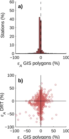
The GIS-polygon dataset was compared to the stations co-registered in DRT. Of these 2177 stations, 2005 were avail-able in the GIS dataset. The GIS-polygon-based basin ar-eas showed small errors compared to those of the gridded dataset, but some stations exhibited markedly large errors (Fig. 5a). As before, the errors showed little consistency be-tween datasets (Fig. 5b). Visual inspection of the mapped area discrepancies of the datasets revealed no geographical pattern for any of the datasets.

4.2 Evaluation of consistency between forcing and evaluation data

Long-term runoff coefficients could be calculated for 1561 of the 2005 stations that were available in both the polygon dataset and in DRT, given that there should be at least 10 yr of consecutive data. To minimise the effect of area discrep-ancies, results shown are based on the GIS-polygon basin delineation. The scatter plot of GPCC and CRU precipita-tion data (Fig. 6a) shows a higher relative difference in pre-cipitation in drier basins. Runoff coefficients for the differ-ent precipitation datasets generally show higher relative dis-crepancies for high runoff coefficients, and implausibly high RCs were mainly found in areas with relatively low precip-itation (Fig. 6b–c). The general distributions of RCs did not differ much between the precipitation datasets, and implau-sibly high runoff coefficients were found for all four datasets even when using the low discharge estimate (Fig. 7). How-ever, RCs higher than one were more common for the CRU and WATCHCRUprecipitation datasets than for the other two.

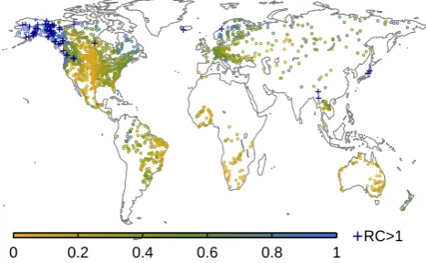
Basins with high runoff coefficients were almost exclusively located in high-latitude or high-altitude areas (Fig. 8). The majority of the basins with RCs exceeding unity were found in Alaska and north-western Canada.

Table 2. Percent of basins (based on the GIS-polygon dataset) exhibiting potential data inconsistencies. Each basin is only accounted for in

the worst category that applies to it, e.g. a basin for which the lowest of the actual evaporation estimates exceed the potential evaporation is

accounted for in columnEAL> EPbut notEAH> EP.

Precipitation Potential No remark EAL> EP EAH> EP P−RL<0 P−RH<0

evaporation

CRU CRU 85.6 4.5 2.9 3.6 3.4

CRU WATCHPM 71.7 12.2 9.1 3.6 3.4

CRU WATCH_PT 62.6 19.8 10.6 3.6 3.4

−1000 0 100

20 40 60

a)

ε_A DDM30 (%)

Stations (%)

−1000 0 100

20 40 60

b)

ε_A DRT (%)

−1000 0 100

20 40 60

c)

ε_A STN−30p (%)

−100 0 100

−100 −50 0 50 100

ε_A DDM30 (%) ε A

STN−30p (%)

d)

−100 0 100

−100 −50 0 50 100

ε_A DRT (%) εA

DDM30 (%)

e)

−100 0 100

−100 −50 0 50 100

ε_A STN−30p (%) ε A

DRT (%)

f)

Fig. 4. Histograms of relative area differences for 558 basins with stations registered in the three gridded flow networks: (a) DDM30, (b) DRT

and (c) STN-30p. The lower panel shows comparisons of the relative area differences for each basin in the different flow networks.

simplified version of the Budyko, 1974, curve) for all com-binations of precipitation and potential-evaporation datasets. The geographical patterns were similar for all combinations (Fig. 9 and Table 2 exemplify the results for the CRU pre-cipitation). Uncertainty in the runoff is represented in colour coding where red represents basins that exhibit actual evap-oration (P−R) higher than potential evaporation even for the high discharge estimate (i.e. when the calculated actual evaporation is the lowest,EAL) and orange represents basins

with actual evaporation higher than the potential-evaporation values for discharge estimates between the low (i.e. when the estimated actual evaporation is the highest,EAH) and the

high values. One noticeable difference between the different potential-evaporation datasets was the greater frequency of basins exhibiting actual evaporation values higher than the potential-evaporation estimates for the two WATCH datasets compared to the CRU dataset. Implausibly high actual evapo-ration frequently appeared in the Amazon basin for all three

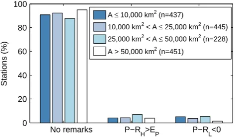
datasets, and for the two WATCH datasets also on the east coast of North America, in Europe, equatorial Africa and South East Asia. Blue dots in Fig. 9 indicate basins for which the actual evaporation was negative (i.e. RC>1) for both the high and low discharge estimates and green dots where this occurred only for the low estimates of actual evapora-tion (i.e. high discharge estimates). The proporevapora-tions of sta-tions with actual evaporation exceeding potential evapora-tion or implausibly high RCs were similar for all basin sizes (Fig. 10).

5 Discussion

5.1 Hydrography representation of basin area

−1000 0 100 10

20 30 40 50 60

Stations (%)

a)

ε_A GIS polygons (%)

−100 −50 0 50 100

−100 −50 0 50 100

ε_A GIS polygons (%)

ε A

DRT (%)

b)

Fig. 5. (a) Relative area differences for 2005 basins based on the

GIS-polygon definition and (b) comparison with relative area dif-ferences exhibited in DRT.

database are likely attributable both to deficiencies in the basin representations, and to varying quality of the GRDC metadata. The accuracy of the areas given in the archive is not reported by the different data providers (U. Looser, head of GRDC, personal communication, October 2011). The larger scatter observed for STN-30p and DRT compared to DDM30 can likely be explained by the extensive manual corrections of the flow network (35 % of all cells) performed on the lat-ter (D¨oll and Lehner, 2002). DDM30 outperforms both STN-30p and DRT in representing basin areas close to the ones re-ported in GRDC (at least for basins larger than 10 000 km2). The advantage of DRT over the other two gridded hydro-graphies would be the possibility to use the high-resolution baseline to derive topographic basin information.

Some of the basin areas reported in the GRDC archive in June 2011 are likely to be different to the ones reported at the time of collection of data for co-registration with STN-30p (Fekete et al., 2002) and DDM30 (Hunger and D¨oll, 2008) since the GRDC archives have been continuously updated. A comparison of Fig. 5 in D¨oll and Lehner (2002) and Fig. 4 in this paper showed that at least a few basin areas must have been updated since no absolute relative area differences above 30 % are reported for the DDM30 stations. Hence, the consistency in errors between DDM30 and STN-30p noted for a few largely over- and underestimated basin areas is an

indication that those stations had different basin areas re-ported in the GRDC archive when those co-registrations were done compared to the archive on 15 June 2011 (when data were collected for this study). Changes in the reported areas were also found between October 2010 (the time of data col-lection for the GIS polygon dataset) and the time when data were collected for this study. The changes were small in most cases, but increases in basin area over 100 % were noted for a few stations.

The GIS-polygon delineation of basins matched basin ar-eas in the GRDC archive well in most cases, but there were some clear discrepancies. Given the extensive manual checks to verify station locations and basin areas during the devel-opment of the dataset, it can be argued that the GIS dataset is more likely correct in case of discrepancy. The area discrep-ancies showed no geographical pattern, even though the GIS dataset is based on a coarser hydrography above 60◦_{N and}

therefore could be expected to perform worse in those areas. Among the 2005 stations common between the GIS dataset and the stations co-registered with DRT, 584 stations had a basin area of 10 000 km2or less. Of those, 80 % exhib-ited relative area differences with absolute values less than 25 % in the gridded hydrography compared to 92 % in the GIS delineation. Corresponding figures for relative area dif-ferences below 10 % were 45 and 84 %, respectively. Hence, many small basin areas were well represented even in the DRT 0.5◦ grid. Basin area was the only means of compari-son in this study, however, even if the relative area difference is small, it does not mean that the spatial extent (shape) of a basin is correctly described and further checks on this is-sue could be made. Uncertainty in the spatial representation is likely to be most pronounced for small basins, and when using gridded instead of GIS-polygon hydrographic datasets.

5.2 Consistency between forcing and evaluation data

0 2 4 0

1 2 3 4

RC

GP

C

C

(−)

RC CRU (−) b)

0 2000 4000

0 1000 2000 3000 4000

P GP

C

C

(mm / year)

P

CRU (mm / year) a)

0 2000 4000

0 1 2 3 4

RC

CRU

(−)

P

CRU (mm/year) c)

Fig. 6. (a) Relation between GPCC and CRU precipitation, (b) best RC estimates based on GPCC precipitation versus CRU precipitation,

and (c) best RC estimates based on CRU precipitation versus CRU precipitation. The 45◦lines indicate the 1:1 quotient and the dashed line

indicate RC = 1.

0 100 200 300 400 500 600

RC (−)

No of stations

≤0.2 0.2−0.4 0.4−0.6 0.6−0.8 0.8−1.0 ≥1 CRU GPCC WATCH

CRU WATCH

GPCC

Fig. 7. Distribution of low-estimate RCs for the four precipitation

datasets.

WATCH precipitation datasets have been corrected for solid undercatch. Hence, the results indicate that those corrections might not be sufficient, assuming that the discharge data can be trusted.

The evaluation of actual and potential evaporation pointed to further inconsistencies between climate and discharge data. Data inconsistencies led to transgression of the potential-evaporation limit (i.e. EA> EP) in many basins.

Peel et al. (2010) report similar issues when analysing a large set (n= 861) of basins worldwide using observed sta-tion records rather than gridded data. Basins exhibiting ac-tual evaporation higher than potential evaporation were more abundant and appeared in more regions when potential evap-oration from the WATCH rather than the CRU dataset was used. Such inconsistencies could be possible for individual basins as a result of e.g. irrigation and inter-basin trans-fers, not accounted for here. However, a main reason for these inconsistencies is likely limitations of the potential-evaporation estimates.

It is common in GHMs to use potential-evaporation estimates that do not explicitly consider vegetation type (e.g. D¨oll et al., 2003; Fekete et al., 1999; Wid´en-Nilsson

+RC>1

0 0.2 0.4 0.6 0.8 1

Fig. 8. Spatial pattern of runoff coefficients for CRU precipitation.

Circles represent best RC estimates and crosses represent basins with low RC estimates higher than one.

0 1000 2000 −1000

0 1000 2000

P−R (mm/year)

CRU E

p(mm/year)

CRU E_p

0 1000 2000

−1000 0 1000 2000

P−R (mm/year)

WATCH_PM E_p (mm/year)

WATCH

PM Ep

0 1000 2000

−1000 0 1000 2000

P−R (mm/year)

WATCH

PT Ep (mm/year)

WATCH_PT E_p

No remark E

AL=P−RH>EP EAH=P−RL>EP P−RL<0 P−RH<0 1:1 line

Fig. 9. Mean annual actual evaporation (estimated asP−Rusing CRU precipitation data) versus potential evaporation from CRU, WATCH Penman–Monteith and WATCH Priestley–Taylor (left panel). Potential evaporation is plotted against actual evaporation estimated using the

best runoff estimate, i.e. theyvalue of each dot represents the best evaporation estimate. The colour coding is based on the high runoff

estimate (RH, giving low estimate ofEA) and low runoff estimate (RL, giving high estimate ofEA) as indicated in the legend. The right

panel shows geographical distributions.

this study were all calculated using data of 0.5◦spatial reso-lution. The real-world variability can be very large within a cell, and because of limited base data, the average cell val-ues may be badly captured both in the input data and in the resulting potential-evaporation estimates. Even if increasing the potential evaporation estimates by 25 %, which would correspond to a very high crop factor in all seasons (Allen et al., 1998), many basins still exhibit actual evaporation higher than the potential evaporation.

0 20 40 60 80 100

Stations (%)

No remarks P−R

H>EP P−RL<0

A ≤ 10,000 km2 (n=437)

10,000 km2 < A ≤ 25,000 km2 (n=445)

25,000 km2 < A ≤ 50,000 km2 (n=228)

A > 50,000 km2 (n=451)

Fig. 10. Basins with and without data inconsistencies, based on

CRU precipitation and potential evaporation, in different area categories.

those issues (e.g. gauge-measurement corrections, surface-dependent estimation of potential evaporation, and consid-eration of anthropogenic influences), and we hope that such studies will follow. As many as 8–43 % of all basins exhib-ited inconsistencies for the best runoff estimate depending on how the datasets were combined. The corresponding fig-ures were 6–35 % when accounting conservatively for dis-charge uncertainties and only counting basins falling com-pletely outside of the physically reasonable limits.

These violations to fundamental consistency assumptions pose a serious problem for model calibration and evalua-tion (Beven and Westerberg, 2011; Beven et al., 2011), and could cause bias in a subsequent model regionalisation. De-pending on the evaluation criteria for the calibration, some of these problems could go unnoticed, but model-parameter values could be biased as a result of such long-term incon-sistencies. It should be noted that there might be periods of informative data in a dataset even if a long-term aver-age is disinformative. Conversely, datasets found consistent in this analysis might contain data that are disinformative on short timescales. There is a need to develop methods to reli-ably identify inconsistent events at short timescales for large spatial-scale datasets.

6 Concluding remarks

This study has demonstrated that a pre-modelling data anal-ysis should be an important first step in a large-scale hydro-logical study. Scrutinising input and evaluation data is vital to reveal inconsistencies between datasets and to highlight basins where one should be cautious when making model in-ferences based on these data. It could be concluded that

– a majority of basins with areas larger than 5000 km2

could be well represented (absolute relative area dif-ference ≤25 %) in a 0.5◦×0.5◦ longitude-latitude grid. The GIS-polygon delineation derived from a

high-resolution hydrographic baseline outperformed the gridded delineation (DRT).

– large and frequent inconsistencies between climate

datasets and observed discharge showed clear spatial patterns. Because of this, it was hypothesised that the inconsistencies were mainly caused by limitations in the forcing/evaluation data. Some inconsistencies could also have been caused by anthropogenic influences not considered in this study (e.g. inter-basin transfers, irri-gation and reservoirs).

In light of the first point, it could be argued that global hydro-logical models should use polygon-based basin delineations rather than limiting delineation accuracy to the resolution of the input data, as is common today. This is especially true since large area discrepancies in coarse flow networks can compensate (or aggravate) precipitation-input deficiencies. Even if a model can perform well in such basins, it might be for the wrong reasons. However, this would require devel-opment of polygon delineations with full global coverage.

In light of the second point, some inconsistencies may be solved by considering sub-grid variability in climate data, surface-dependent potential-evaporation estimates, etc., but it is likely that inconsistencies for many basins cannot be re-solved based on available global data. Further studies will be required to find out the reasons for these inconsistencies and how they affect model inference. A model-independent data analysis, such as the one presented in this study, is a useful tool to identify and analyse inconsistent datasets – therefore enabling more robust conclusions in subsequent hydrological modelling and analyses (Juston et al., 2012).

Acknowledgements. This study has been heavily dependent on

provision of global datasets provided by several groups mentioned in the data section. We would like to thank all the groups that have been involved in the development of those datasets. Special thanks are extended to Huan Wu who provided the early version of the DRT dataset, to Petra D¨oll who provided the DDM30 dataset, and to the helpful staff at GRDC. The authors are grateful to Keith Beven, Dai Yamazaki and one anonymous reviewer for their constructive comments on the original manuscript.

Edited by: F. Pappenberger

References

Adam, J. C. and Lettenmaier, D. P.: Adjustment of global gridded precipitation for systematic bias, J. Geophys. Res., 108, 4257, doi:10.1029/2002JD002499, 2003.

Allen, R. G., Smith, M., Pereira, L. S., and Perrier, A.: An update for the calculation of reference evapotranspiration, ICID Bull., 43, 35–92, 1994.

Arnell, N. W.: A simple water balance model for the simulation of streamflow over a large geographic domain, J. Hydrol., 217, 314–335, 1999a.

Arnell, N. W.: Climate change and global water resources, Global Environ. Change, 9, 31–49, 1999b.

Aronica, G. T., Candela, A., Viola, F., and Cannarozzo, M.: Influ-ence of rating curve uncertainty on daily rainfall-runoff model predictions, in: Predictions in Ungauged Basins: Promise and Progress, edited by: Sivapalan, M., Wagener, T., Uhlenbrook, S., Liang, X., Lakshmi, V., Kumar, P., Zehe, E., and Tachikawa, Y., IAHS Publ., 303, 116–124, 2006.

BADC: http://badc.nerc.ac.uk/view/badc.nerc.ac.ukATOMdataent 1256223773328276, last access: 8 March 2013.

Becker, A., Finger, P., Meyer-Christoffer, A., Rudolf, B., Schamm, K., Schneider, U., and Ziese, M.: A description of the global land-surface precipitation data products of the Global Precipita-tion Climatology Centre with sample applicaPrecipita-tions including cen-tennial (trend) analysis from 1901–present, Earth Syst. Sci. Data, 5, 71–99, doi:10.5194/essd-5-71-2013, 2013.

Beven, K. and Westerberg, I.: On red herrings and real herrings: dis-information and dis-information in hydrological inference, Hydrol. Process., 25, 1676–1680, 2011.

Beven, K., Smith, P. J., and Wood, A.: On the colour and spin of epistemic error (and what we might do about it), Hy-drol. Earth Syst. Sci., 15, 3123–3133, doi:10.5194/hess-15-3123-2011, 2011.

Budyko, M. I.: Climate and Life, International Geophysics Se-ries No. 18, edited by: Miller, D. H., Academic Press, London, 508 pp., 1974.

Decharme, D. and Douville, H.: Uncertainties in the GSWP-2 pre-cipitation forcing and their impacts on regional and global hy-drological simulations, Clim. Dynam., 27, 695–713, 2006. D¨oll, P. and Lehner, B.: Validation of a new global 30-min drainage

direction map, J. Hydrol., 258, 214–231, 2002.

D¨oll, P. and Siebert, S.: Global modeling of irrigation water require-ments, Water Resour. Res., 38, 1037–1045, 2002.

D¨oll, P., Kaspar, F., and Lehner, B.: A global hydrological model for deriving water availability indicators: model tuning and vali-dation, J. Hydrol., 270, 105–134, 2003.

Fekete, B. M., V¨or¨osmarty, C. J., and Grabs, W.: Global composite runoff fields of observed river discharge and simulated water bal-ances, Tech. Rep. No. 22, Global Runoff Data Centre, Koblenz, Germany, 39 pp. plus Annex, 1999.

Fekete, B. M., V¨or¨osmarty, C. J., and Grabs, W.: High-resolution fields of global runoff combining observed river discharge and simulated water balances, Global Biogeochem. Cy., 16, 1042, doi:10.1029/1999GB001254, 2002.

Fekete, B. M., V¨or¨osmarty, C. J., Roads, J. O., and Willmott, C. J.: Uncertainties in precipitation and their impacts on runoff esti-mates, J. Climate, 17, 294–304, 2004.

Freer, J. E., McMillan, H., McDonnell, J. J., and Beven, K. J.: Con-straining dynamic TOPMODEL responses for imprecise water table information using fuzzy rule based performance measures, J. Hydrol., 291, 254–277, doi:10.1016/j.jhydrol.2003.12.037, 2004.

Gong, L., Halldin, S., and Xu, C.-Y.: Global-scale river rout-ing – an efficient time-delay algorithm based on HydroSHEDS high-resolution hydrography, Hydrol. Process., 25, 1114–1128, doi:10.1002/hyp.7795, 2011.

Gosling, S. N. and Arnell, N. W.: Simulating current global river runoff with a global hydrological model: model revisions, vali-dation, and sensitivity analysis, Hydrol. Process., 25, 1129–1145, doi:10.1002/hyp.7727, 2011.

G¨untner, A.: Improvement of global hydrological models using GRACE data, Surv. Geophys., 29, 375-397, 2008.

Hagemann, S., Arpe, K., and Bengtsson, L.: Validation of the hy-drological cycle of ERA-40, Reports on earth system science, Max Planck Institute, Hamburg, Germany, 2005.

Hanasaki, N., Kanae, S., Oki, T., Masuda, K., Motoya, K., Shi-rakawa, N., Shen, Y., and Tanaka, K.: An integrated model for the assessment of global water resources – Part 1: Model descrip-tion and input meteorological forcing, Hydrol. Earth Syst. Sci., 12, 1007–1025, doi:10.5194/hess-12-1007-2008, 2008. Harris, I., Jones, P. D., Osborn, T. J., and Lister, D. H.: Updated

high-resolution grids of monthly climatic observations – the CRU TS3.10 Dataset, Int. J. Climatol., doi:10.1002/joc.3711, in press, 2013.

Hunger, M. and D¨oll, P.: Value of river discharge data for global-scale hydrological modeling, Hydrol. Earth Syst. Sci., 12, 841– 861, doi:10.5194/hess-12-841-2008, 2008.

Jung, G., Wagner, S., and Kunstmann, H.: Joint climate-hydrology modeling: an impact study for the data-sparse environment of the Volta Basin in West Africa, Hydrol. Res., 43, 231–248, 2012. Juston, J. M., Kauffeldt, A., Quesada Montano, B., Seibert, J.,

Beven, K., and Westerberg, I.: Smiling in the rain: Seven rea-sons to be positive about uncertainty in hydrological modelling, Hydrol. Process., 27, 1117–1122, doi:10.1002/hyp.9625, 2012. Kaspar, F.: Entwicklung und unsicherheitanalyse eines globalen

hy-drologischen modells, Ph.D. Thesis, Department of Natural Sci-ences, Kassel University, Kassel, Germany, 139 pp., 2004. Kuczera, G.: Correlated rating curve error in flood frequency

infer-ence, Water Resour. Res., 32, 2119–2127, 1996.

Lehner, B.: Derivation of watershed boundaries for GRDC gaug-ing stations based on the HydroSHEDS drainage network, Tech. Rep. No. 41, Global Runoff Data Centre, Koblenz, Ger-many, 12 pp., 2011.

Lehner, B., Verdin, K., and Jarvis, A.: New global hydrography de-rived from spaceborne elevation data, Eos. Trans. AGU, 89, 93, 2008.

Li, L., Ngongondo, C. S., Xu, C.-Y., and Gong, L.: Comparison of the global TRMM and WFD precipitation datasets in driving a large-scale hydrological model in Southern Africa, Hydrol. Res., doi:10.2166/NH.2012.175, in press, 2012.

McMillan, H., Krueger, T., and Freer, J.: Benchmarking ob-servational uncertainties for hydrology: rainfall, river dis-charge and water quality, Hydrol. Process., 26, 4078–4111, doi:10.1002/HYP.9384, 2012.

Mitchell, T. D. and Jones, P. D.: An improved method of construct-ing a database of monthly climate observations and associated high-resolution grids, Int. J. Climatol., 25, 693–712, 2005. Montanari, A. and Di Baldassarre, G.: Data errors and

hydro-logical modelling: The role of model structure to propagate observation uncertainty, Adv. Water Resour., 51, 498–504, doi:10.1016/j.advwatres.2012.09.007, 2012.

Mulligan, M.: WaterWorld: a self-parameterising, physically-based model for application in data-poor but problem-rich environ-ments globally, Hydrol. Res., doi:10.2166/nh.2012.217, in press, 2012.

New, M., Hulme, M., and Jones, P.: Representing twentieth-century space–time climate variability, Part I: Development of a 1961–90 mean monthly terrestrial climatology, J. Climate, 12, 829–856, 1999.

Nijssen, B., O’Donnell, G., Hamlet, A., and Lettenmaier, D.: Hy-drologic sensitivity of global rivers to climate change, Climatic Change, 50, 143–175, 2001.

Palmer, M. A., Reidy Liermann, C. A., Nilsson, C., Fl¨orke, M., Alcamo, J., Lake, P. S., and Bond, N.: Climate change and the world’s river basins: anticipating management options, Front. Ecol. Environ., 6, 81–89, 2008.

Peel, M. C., McMahon, T. A., and Finlayson, B. L.: Veg-etation impact on mean annual evapotranspiration at a global catchment scale, Water Resour. Res., 46, W09508, doi:10.1029/2009WR008233, 2010.

Priestley, C. H. B. and Taylor, R. J.: On the assessment of surface heat flux and evaporation using large-scale parameters, Mon. Weather Rev., 100, 81–92, 1972.

Strasser, U., Bernhardt, M., Weber, M., Liston, G. E., and Mauser, W.: Is snow sublimation important in the alpine water balance?, The Cryosphere, 2, 53–66, doi:10.5194/tc-2-53-2008, 2008. Thyer, M., Renard, B., Kavetski, D., Kuczera, G., Franks, S. W.,

and Srikanthan, S.: Critical evaluation of parameter consistency and predictive uncertainty in hydrological modeling: A case study using Bayesian total error analysis, Water Resour. Res., 45, W00b14, doi:10.1029/2008WR006825, 2009.

Uppala, S. M., K˚allberg, P. W., Simmons, A. J., Andrae, U., Bech-told, V. D. C., Fiorino, M., Gibson, J. K., Haseler, J., Hernandez, A., Kelly, G. A., Li, X., Onogi, K., Saarinen, S., Sokka, N., Allan, R. P., Andersson, E., Arpe, K., Balmaseda, M. A., Beljaars, A. C. M., Berg, L. V. D., Bidlot, J., Bormann, N., Caires, S., Chevallier, F., Dethof, A., Dragosavac, M., Fisher, M., Fuentes, M., Hage-mann, S., H´olm, E., Hoskins, B. J., Isaksen, L., Janssen, P. A. E. M., Jenne, R., Mcnally, A. P., Mahfouf, J.-F., Morcrette, J.-J., Rayner, N. A., Saunders, R. W., Simon, P., Sterl, A., Trenberth, K. E., Untch, A., Vasiljevic, D., Viterbo, P., and Woollen, J.: The ERA-40 re-analysis, Q. J. Roy. Meteorol. Soc., 131, 2961–3012, doi:10.1256/qj.04.176, 2005.

USGS EROS, HYDRO1k Elevation Derivative Database:

http://eros.usgs.gov/#/FindData/Products andDataAvailable/ gtopo30/hydro (last access: 30 September 2012), 1996. V¨or¨osmarty, C. J., Moore III, B., Grace, A. L., Gildea, M. P.,

Melillo, J. M., Peterson, B. J., Rastetter, E. B., and Steudler, P. A.: Continental scale models of water balance and fluvial trans-port: An application to South America, Global Biogeochem. Cy., 3, 241–265, 1989.

V¨or¨osmarty, C. J., Fekete, B. M., Meybeck, M., and Lammers, R. B.: Global system of rivers: Its role in organizing continental land mass and defining land-to-ocean linkages, Global Biogeochem. Cy., 14, 599–621, 2000.

Vrugt, J. A., ter Braak, C. J. F., Clark, M. P., Hyman, J. M., and Robinson, B. A.: Treatment of input uncertainty in hy-drologic modeling: Doing hydrology backward with Markov chain Monte Carlo simulation, Water Resour. Res., 44, W00B09, doi:10.1029/2007WR006720, 2008.

Weedon, G. P., Gomes, S., Viterbo, P., Shuttleworth, W. J., Blyth,

E., ¨Osterle, H., Adam, J. C., Bellouin, N., Boucher, O., and Best,

M.: Creation of the WATCH forcing data and its use to assess global and regional reference crop evaporation over land during the twentieth century, J. Hydrometeorol., 12, 823–848, 2011. Werth, S. and G¨untner, A.: Calibration analysis for water storage

variability of the global hydrological model WGHM, Hydrol. Earth Syst. Sci., 14, 59–78, doi:10.5194/hess-14-59-2010, 2010. Westerberg, I. K., Guerrero, J.-L., Younger, P. M., Beven, K. J., Seibert, J., Halldin, S., Freer, J. E., and Xu, C.-Y.: Calibra-tion of hydrological models using flow-duraCalibra-tion curves, Hy-drol. Earth Syst. Sci., 15, 2205–2227, doi:10.5194/hess-15-2205-2011, 2011.

Wid´en-Nilsson, E., Halldin, S., and Xu, C.-Y.: Global water-balance modelling with WASMOD-M: Parameter estimation and region-alisation, J. Hydrol., 340, 105–118, 2007.

Wid´en-Nilsson, E., Gong, L., Halldin, S., and Xu, C.-Y.: Model performance and parameter behavior for varying time aggre-gations and evaluation criteria in the WASMOD-M global water balance model, Water Resour. Res., 45, W05418, doi:10.1029/2007WR006695, 2009.

Wisser, D., Frolking, S., Douglas, E. M., Fekete, B. M., V¨or¨osmarty, C. J., and Schumann, A. H.: Global irrigation water de-mand: Variability and uncertainties arising from agricultural and climate data sets, Geophys. Res. Lett., 35, L24408, doi:10.1029/2008GL035296, 2008.

Wisser, D., Fekete, B. M., V¨or¨osmarty, C. J., and Schumann, A. H.: Reconstructing 20th century global hydrography: a contribution to the Global Terrestrial Network-Hydrology (GTN-H), Hydrol. Earth Syst. Sci., 14, 1–24, doi:10.5194/hess-14-1-2010, 2010. Wu, H., Kimball, J. S., Mantua, N., and Stanford, J.: Automated

up-scaling of river networks for macroscale hydrological modeling, Water Resour. Res., 47, W03517, doi:10.1029/2009WR008871, 2011.

Wu, H., Kimball, J. S., Li, H., Huang, M., Leung, L. R., and Adler, R. F.: A new global river network database for macroscale hydrologic modeling, Water Resour. Res., 48, W09701, doi:10.1029/2012WR012313, 2012.

Yamazaki, D., Oki, T., and Kanae, S.: Deriving a global river net-work map and its sub-grid topographic characteristics from a fine-resolution flow direction map, Hydrol. Earth Syst. Sci., 13, 2241–2251, doi:10.5194/hess-13-2241-2009, 2009.