Modelling of the shallow water table at high spatial resolution using random forests

https://doi.org/10.5194/hess-23-4603-2019 © Author(s) 2019. This work is distributed under the Creative Commons Attribution 4.0 License.

Modelling of the shallow water table at high spatial

resolution using random forests

Julian Koch1, Helen Berger2, Hans Jørgen Henriksen1, and Torben Obel Sonnenborg1

1_{Department of Hydrology, Geological Survey of Denmark and Greenland (GEUS), Copenhagen, 1350, Denmark} 2_{COWI A/S, Lyngby, 2800, Denmark}

Correspondence:Julian Koch ([email protected])

Received: 1 May 2019 – Discussion started: 10 May 2019

Revised: 11 September 2019 – Accepted: 8 October 2019 – Published: 15 November 2019

Abstract. Machine learning provides great potential for modelling hydrological variables at a spatial resolution be-yond the capabilities of physically based modelling. This study features an application of random forests (RF) to model the depth to the shallow water table, for a wintertime mini-mum event, at a 50 m resolution over a 15 000 km2domain in Denmark. In Denmark, the shallow groundwater poses se-vere risks with respect to groundwater-induced flood events, affecting both urban and agricultural areas. The risk is espe-cially critical in wintertime, when the shallow groundwater is close to terrain. In order to advance modelling capabilities of the shallow groundwater system and to provide estimates at the scales required for decision-making, this study introduces a simple method to unify RF and physically based modelling. Results from the national water resources model in Denmark (DK-model) at a 500 m resolution are employed as covariates in the RF model. Thus, RF ensures physical consistency at a coarse scale and fully exhausts high-resolution information from readily available environmental variables. The vertical distance to the nearest water body was rated as the most im-portant covariate in the trained RF model followed by the DK-model. The evaluation test of the trained RF model was very satisfying with a mean absolute error of 76 cm and a co-efficient of determination of 0.56. The resulting map under-lines the severity of groundwater flooding risk in Denmark, as the average depth to the shallow groundwater is 1.9 m and approximately 29 % of the area is characterized as having a depth of less than 1 m during a typical wintertime minimum event. This study brings forward a novel method for assess-ing the spatial patterns of covariate importance of the RF pre-dictions that contributes to an increased interpretability of the RF model. Quantifying the uncertainty of RF models is still

rare for hydrological applications. Two approaches, namely random forests regression kriging (RFRK) and quantile re-gression forests (QRF), were tested to estimate uncertainties related to the predicted groundwater levels.

1 Introduction

The shallow groundwater, defined as the uppermost water ta-ble, is a key state variable of the hydrological cycle that has a wide range of vital implications for human health, terrestrial ecosystems, food security and energy production (Gleeson et al., 2016). Following Fan et al. (2013), up to one-third of the global land area is affected by shallow groundwater, being either directly groundwater-fed or having the water table or capillary fringe within plant rooting depths. In many regions of the world, groundwater aquifers are being depleted ex-tensively by unsustainable anthropogenic activities (Richey et al., 2015). In addition, climate change affects groundwa-ter recharge and storage, which, in many cases, impacts the resilience of shallow groundwater systems (Ferguson and Maxwell, 2010; Rodell et al., 2018).

wa-ter table has on the energy balance at the land surface, infer-ring a link to the latent heat flux and the delineation of water-and energy-limited ecosystems (Kollet water-and Maxwell, 2008; Maxwell and Condon, 2016). Other studies stressed the con-nections between groundwater and the near-surface climate via coupled numerical modelling experiments (Larsen et al., 2016; Wang et al., 2018). Shallow groundwater is also of im-portance in urban contexts (Bricker et al., 2017), with special focus on urban flooding which can be directly induced or indirectly intensified by high groundwater levels (Jankowf-sky et al., 2014; Kreibich and Thieken, 2008; MacDonald et al., 2012). Moreover, MacDonald et al. (2010) and Upton and Jackson (2011) studied the underlying processes, esti-mated return periods and mapped risk of groundwater flood-ing events.

In Denmark, the quantitative status of shallow groundwa-ter systems is challenged by climate change and groundwagroundwa-ter abstraction (Henriksen et al., 2008; Karlsson et al., 2016). In more detail, Kidmose et al. (2013) demonstrated that ground-water levels are expected to rise by up to 1.5 m for a 100-year event relative to present average conditions. Similar findings were presented by van Roosmalen et al. (2007), who quan-tified regional differences across Denmark in the projected change of groundwater levels depending on soil types with more profound increases in highly permeable sandy soils. Moreover, Henriksen et al. (2012) analysed climate change effects on the shallow water table over Denmark for mean and maximum conditions for nine different climate models and identified changes of at least 0.5 m for 26 % of Denmark. This finding represented the median change across the nine applied climate models.

The above-mentioned problems call for comprehensive modelling tools that can support environmental decision-making aiming at tackling current and future challenges re-lated to shallow groundwater. Spatial scales that are rele-vant for society and required for adequate decision-making can typically not be provided by numerical, physically based models alone. This limitation is mainly related to the fact that such models are computationally very expensive which hinders thorough conduct calibration, sensitivity and uncer-tainty analysis at high resolution (Asher et al., 2015; Stisen et al., 2018). Furthermore, it is difficult to parameterize sub-surface processes regardless the scale (Beven et al., 2015). Moreover, the wealth and detail of hydrological data are un-der continual growth (Chaney et al., 2018) and the resulting big data are often not harnessed optimally in existing mod-elling frameworks (Best et al., 2015; Nearing et al., 2016). As outlined by Reichstein et al. (2019), machine learning will play an essential role in advancing current modelling sys-tems by integrating machine learning and numerical models. The development and testing of such hybrid models, com-plementing the benefits of physically based models and ma-chine learning, have gradually gained more attention in re-cent years in the hydrological community. A roadmap toward machine-learning-facilitated discoveries of hydrological

sys-tems has been outlined by Shen at al. (2018) and will likely play an eminent role in the future of hydrology. More gen-erally, Karpatne et al. (2017) coined the paradigm “theory-guided data science” which comprises a diverse list of ap-proaches with which physically based models and machine learning can be combined. All three of the above-mentioned references focus on the coupling of physically based models with the versatility of data-driven modelling frameworks. In more detail, they have identified that the interpretability of machine learning models is among the main challenges for the successful adoption of big data technologies in hydrolog-ical science.

This study highlights the applicability of machine learn-ing, namely the random forests (RF) algorithm (Breiman, 2001), to model the depth to the shallow groundwater at a re-gional scale at high spatial resolution. The aim is to produce a map that captures an extreme wintertime condition, repre-senting a minimum depth to the water table. Such an event can potentially induce groundwater flooding that poses risks related to infrastructure and agriculture. Thus, the resulting high-resolution map will be a versatile screening resource for environmental decision-making and climate change adaption planning. The proposed RF model draws on the Danish na-tional water resources model (Højberg et al., 2013) which provides a coarse estimation of the depth to the shallow wa-ter table. In this way, the RF model utilizes the coarse pre-diction of the physically based model to ensure overall phys-ical consistency, which may not be granted by the RF model alone. Hence, this study tests a simple hybrid model integrat-ing the output of a numerical model in a machine learnintegrat-ing framework. Before machine learning techniques can be con-sidered as a standard tool for environmental decision-making and planning, methods to conduct comprehensive sensitiv-ity analysis and uncertainty assessment need to be developed and tested thoroughly. In order to advance this field of hydro-logical research, this study compares two different methods for quantifying the uncertainty of a RF model, namely ran-dom forests regression kriging (Hengl et al., 2015) and quan-tile regression forests (Meinshausen, 2006). Furthermore, this study features a novel methodology to quantify covariate importance, and thereby the sensitivity of the model inputs, which ultimately helps to better comprehend and interpret the RF prediction.

groundwater-related variables, such as the nitrate concentra-tion (Nolan et al., 2015; Tesoriero et al., 2015), arsenic con-centrations (Erickson et al., 2018; Winkel et al., 2011) and redox conditions in the subsurface (Close et al., 2016; Koch et al., 2019), and the potential to map the depth to the water table is tangible.

The four main objectives of this paper are as follows: (1) to train a RF model that is capable of predicting the depth to the shallow water table at a high spatial resolution, (2) to outline a simple and generic method that unifies a physically based model and machine learning, (3) to conduct a comprehensive sensitivity analysis to better interpret the RF model predic-tion and (4) to assess the uncertainty related to the RF model based on two different approaches.

2 Methods 2.1 Study area

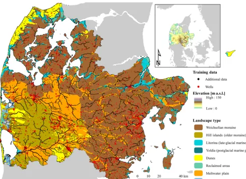
The study area encompasses a large part of the Jutland Peninsula, which is located in Denmark in northern Europe (54.5–57.8◦N and 8.0–10.9◦E). The extent of the study area amounts to approximately 15 000 km2and its general surfi-cial geological setting is illustrated in Fig. 1. The landscape of Jutland was formed by a sequence of Pleistocene glacia-tions and postglacial processes. The geology of the east-ern part of the study domain is dominated by Weichselian moraine sediments with a moderate clay content, whereas the west is characterized by moraine sediments originating from the Saalian age, referred to as hill islands, intertwined by sandy Weichselian outwash plains.

2.2 Data

This study aims at modelling the depth to the shallow water table at a 50 m spatial resolution using a machine learning modelling framework. Disregarding the prevailing temporal variability of groundwater dynamics close to the surface, we chose to model an extreme event that characterizes a mini-mum depth which is expected to arise every year. Based on the climate in Denmark, such an event normally occurs to-wards the end of winter, when shallow aquifer systems are replenished after several months of typically high rainfall and low evapotranspiration. Applying machine learning to model an extreme event of a highly dynamic variable poses distinct challenges to the training dataset. Long time series of groundwater head measurements are scarce, and shallow groundwater time series are even more rare. In fact, many shallow wells, with screens within the uppermost 10 m, pro-vide just one to a few observations in total. In order to cap-italize on these low-frequency sampled wells, we developed a method to transform any given observations to an expected high water table. For this transformation, sinus curves were defined with varying amplitudes that captured the annual

dy-namics of the shallow groundwater for various hydrogeolog-ical settings. The workflow is described in more detail below. First, well data, covering the entire model domain, were extracted from the national database, Jupiter (Hansen and Pjetursson, 2011). Groundwater head observations from wells with a maximum filter depth of 10 m were assorted for a 20-year period between 1998 and 2017. Several con-straints were applied to this initial extraction: (1) the mean water level may not be below the filter depth, (2) the water levels may not exceed 5 m above the surface, (3) the stan-dard deviation of the head observations may not be greater than 3 m and (4) the well may not be in operation. By ap-plying these four constraints, 14 916 wells with one or more head observations were selected which approximately corre-sponds to a density of one well per square kilometre. Figure 1 shows the location of the wells.

Second, wells with more than five observations, of which 392 were present, were grouped according to their hydroge-ological setting. Subsequently, their standard deviation was studied in more detail in order to define the sinus curve am-plitudes for each of the groups. In total, 27 combinations, de-scribing the general hydrogeological setting of a well, were assessed. These groups were based on three categories with three subcategories each, (1) permeability (high, low or known), (2) aquifer condition (confined, unconfined or un-known) and (3) proximity (near the coastline, near stream or other). The amplitude of the sinus curve was set to the 99 % confidence interval and, under the assumption of normality, calculated as 2.576 times the standard deviation. Based on the analysis of the variability at 392 wells with long time se-ries the average annual amplitude of the sinus curves varied between 0.5 and 1.5 m depending on the hydrogeological set-ting. The largest amplitude was associated with wells with filters in sediment with low permeability, under unconfined conditions and not in the vicinity of the coastline or streams. Low amplitudes were generally connected with wells closer than 100 m to streams, lakes or the coastline. The minimum and maximum of the sinus curves was set to arise in mid-February and mid-August respectively.

Figure 1.The study site is located in central Denmark. The inset figure is an overview depicting the digital elevation model. The main map shows the predominant geological landscape types. The training dataset contains observations at∼15 000 wells. Additionally,∼16 000 artificial observations, placed along major rivers, lakes and the coastline, are added to the analysis. The depth to the shallow groundwater is set to zero for the additional data.

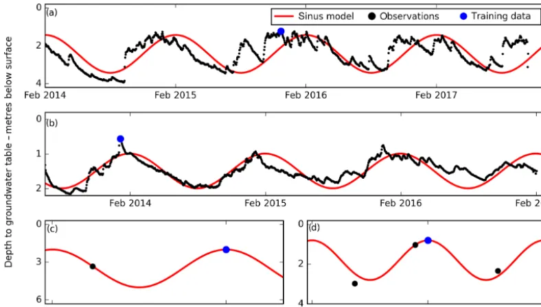
applied to transform the observed minimum depth to an ex-pected winter minimum condition. In cases where the trans-formation resulted in negative values, i.e. manifesting arte-sian conditions, the value was set to zero. This correction was considered meaningful as many of these wells were located in unconfined conditions. The resulting training dataset con-sisted of 14 916 wells; from these wells, 97 % were corrected with sinus curves, and the observed minimum depth was used at the remaining 3 %. Figure 2 indicates that the minimum depths based on the measured values and sinus model may deviate for the 392 wells with long time series. However, the two examples in Fig. 2 imply a deviation of 10–20 cm, which lies within the measurement uncertainty itself. This allows us to conclude that the proposed sinus model-based correction is robust enough for our application.

There are two sources of uncertainty that were not con-sidered in this analysis. First, the observational uncertainty related to the head values in the well database was not taken into account. Second, the sinus model used to traverse any

given observation to an expected wintertime minimum ne-glected seasonal and inter-annual variability.

represen-Figure 2.Four examples showing how the training dataset was derived. At wells with more than four observations(a, b), the minimum daily observation was chosen. Examples(a)and(b)represent long time series and sinus curves with amplitudes of 1 and 0.5 m respectively, and were used to describe the annual variability. Examples(c)and(d)represent two cases with few observations. Here, sinus curves with predefined amplitudes, 1.5 and 1 m respectively, corresponding to the well’s hydrogeological setting were applied to traverse the observed minimum depth to an expected wintertime minimum.

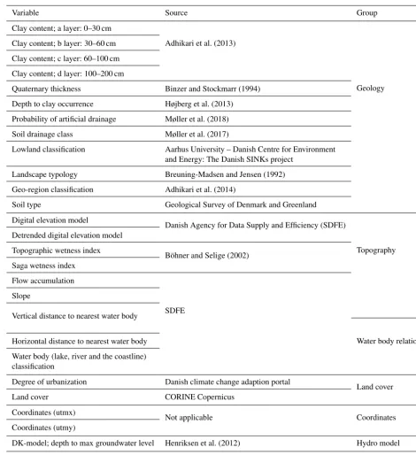
tative for the study site. The complete dataset of additional observations was, however, utilized in the uncertainty anal-ysis. In Table 1, a list of the environmental covariates used to model the depth of the shallow water table is found. In total, 27 covariates were assembled as input to the machine learning model. This list comprises information on soil tex-ture, drainage conditions, geology, topography-based char-acteristics, water body proximity, precipitation, land cover, geographic location and outputs from a hydrological simu-lation with the Danish national water resources model (DK-model; Højberg et al., 2013). The native spatial resolution of the covariates varied, but all covariates were resampled to 50 m to be in agreement with the defined output resolution. The water body proximity was expressed as both the verti-cal and horizontal distance to the nearest water body, which contained rivers, lakes and the coastline. The covariates were subdivided into six groups, i.e. geology, topography, water body relation, precipitation, land cover, coordinates and hy-drological model. This subdivision was implemented in the sensitivity analysis of the machine learning model to elimi-nate correlations between covariates.

2.3 Random forests

This study applied random forests (RF) regression to model the depth to the shallow water table at high spatial res-olution at the regional scale. RF was first proposed by Breiman (2001) and has emerged as a prevalent modelling tool covering a wide range of geophysical and

aver-Table 1.Overview of the covariates used to model the shallow water table using RF.

Variable Source Group

Clay content; a layer: 0–30 cm

Adhikari et al. (2013)

Geology Clay content; b layer: 30–60 cm

Clay content; c layer: 60–100 cm

Clay content; d layer: 100–200 cm

Quaternary thickness Binzer and Stockmarr (1994)

Depth to clay occurrence Højberg et al. (2013)

Probability of artificial drainage Møller et al. (2018)

Soil drainage class Møller et al. (2017)

Lowland classification Aarhus University – Danish Centre for Environment and Energy: The Danish SINKs project

Landscape typology Breuning-Madsen and Jensen (1992)

Geo-region classification Adhikari et al. (2014)

Soil type Geological Survey of Denmark and Greenland

Digital elevation model

Danish Agency for Data Supply and Efficiency (SDFE)

Topography Detrended digital elevation model

Topographic wetness index

Böhner and Selige (2002) Saga wetness index

Flow accumulation

SDFE Slope

Vertical distance to nearest water body

Water body relation Horizontal distance to nearest water body

Water body (lake, river and the coastline) classification

Degree of urbanization Danish climate change adaption portal

Land cover

Land cover CORINE Copernicus

Coordinates (utmx)

Not applicable Coordinates

Coordinates (utmy)

DK-model; depth to max groundwater level Henriksen et al. (2012) Hydro model

Precipitation Danish Meteorological Institute Precipitation

age across the entire ensemble represents the final RF predic-tion. Second, only a subset of the covariates is drawn upon when splitting the data during the process of decision tree building. This subset, usually 33 % of the available covari-ates, is selected randomly for each split. In combination, the two elements of randomness decrease the accuracy of a sin-gle tree; however, the diversity between the trees increases,

which results in a robust prediction when averaging across all trees.

its own oob sample, and the average across all oob predic-tions allows for the quantification of the overall accuracy of the RF model. For the oob prediction, only samples retained from the training, thus out-of-bag samples, are considered when averaging. In this way, the entire ensemble of trees can be evaluated by applying the oob approach. In order to quan-tify the performance of the RF model, we have applied the following metrics on the oob prediction: coefficient of deter-mination (R2), mean absolute error (MAE) and root-mean-squared error (RMSE). We applied the Scikit-learn Python package (Pedregosa et al., 2012) to conduct the RF modelling for this study.

2.4 Covariate sensitivity

The concept of covariate permutation allows one to assess the importance of each covariate that acts as input to a RF model (Biau and Scornet, 2016). This can be understood as a sensitivity analysis which can help to better comprehend and interpret the trained RF model and to gain physical insights into the otherwise nontransparent black-box model. This is achieved by permuting each covariate at a time, while leaving the remaining covariates unchanged, and tracing the apparent decrease in the oob evaluation metric. Typically, the coeffi-cient of determination (R2) is used as a metric, but other met-rics could also be consulted as the sensitivity may be metric dependent. This concept is common practice to assess co-variate importance for a trained RF model (Ließ et al., 2012; Lutz et al., 2018). However, this analysis is limited to the training dataset, and conclusions on which covariates dom-inate the prediction and how this varies spatially cannot be drawn. In order to gain insights into the spatial patterns of covariates’ importance, we have developed a novel method, which applies the above-mentioned concept of covariate per-mutation on the prediction dataset instead of the training dataset. The aim of the sensitivity analysis is to identify a relative ranking of covariate importance for each simulation grid, which can ultimately provide increased interpretability. The starting point of the analysis is the trained RF model and its prediction at all simulation grids. Sequentially, each covariate is permuted, while leaving the remaining covari-ates unchanged, and the trained RF model is used to make a modified prediction. The difference between the modified and original prediction is recorded. The cycle of permuta-tion and predicpermuta-tion is repeated n times until the mean dif-ference acrossnpermutations converges for each simulation grid. This is necessary, because a single permutation may allegedly result in no or minor change in a covariate value at specific grids. Once the mean difference has converged, the covariates can be ranked with respect to their associated mean absolute difference for each simulation grid. In order to map the spatial covariate sensitivity it is essential that the ranking is performed at each simulation grid. This ranking expresses the relative covariate importance and is the key re-sult of the proposed sensitivity analysis. Maps showing the

top ranks can be used to visualize the spatial patterns of the sensitivity of the RF model.

Typically, strong correlations are found between covari-ates, which may result in an alleged low importance when being permuted individually (Koch et al., 2019). In order to overcome this limitation, we suggest a supplementary anal-ysis that collectively permutes groups of covariates that are physically related.

2.5 Random forests regression kriging

Extending RF using geostatistical methods is gaining popu-larity in the field of digital soil mapping (Guo et al., 2015; Hengl et al., 2015) and related environmental modelling studies (Ahmed et al., 2017; Li et al., 2011; Viscarra Rossel et al., 2014). Regression kriging (RK) is a widely applied approach that combines a multiple linear regression (MLR) model with a geostatistical model of the MLR residuals (Hengl et al., 2007; Odeh et al., 1995). In order to integrate RF into RK, RF can simply replace the MLR model. In this way, RF provides an overall data-driven trend and the RF residuals can be interpolated using geostatistics. This results in a hybrid model that is commonly referred to as random forests regression kriging (RFRK). To our knowledge, RFRK has not yet been applied with the purpose of predicting a hy-drological state variable such as groundwater head. RFRK can be expressed by

PRFRK(s0)=TRF(s0)+ ˆeRF(s0) , (1)

whereTRF(s0)is the RF prediction at locations0andeˆRF(s0) is the estimated residual at the same location. The sum of trend (TRF) and residual (eˆRF) yields the final RFRK predic-tion (PRFRK). This study utilizes kriging to interpolate the oob residuals of the RF model. We use the oob prediction instead of the overall RF prediction to compute the resid-uals, because the oob procedure provides a more realistic estimation of the generalization error. The overall RF pre-diction naturally exhibits a lower error than the oob predic-tions as the data were contained in the training. Therefore, the resulting error variance would be biased and can not be used to interpolate the error at unsampled locations. Kriging is a popular geostatistical technique for spatial interpolation that employs knowledge about the spatial autocorrelation of a variable, which can be captured by a variogram model. For the definition of a variogram model, the omnidirectional em-pirical semivariance (γ) is calculated by

γ (h)= 1

2n(h) n(h) X

i=1

[e (si)−e (si+h)]2, (2)

wheren(h)marks the total number of data pairs at a given lag distanceh,e(si)represents the oob residual at locationsi

ande(si+h)is the residual separated by laghfromsi

spatial autocorrelation structure of the oob residuals (Clay-ton and Andre, 1998). The parameters defining a variogram model are type, range, sill and nugget. The Gstat R package (Pebesma, 2004) was applied for variogram modelling and kriging interpolation.

The addition of residual kriging to RF results in high ac-curacy at grids coinciding with observations. Furthermore, kriging quantifies the prediction uncertainty following the defined variogram model. Generally, the kriging variance is low in the vicinity of data points and increases to the sill value once the distance to the nearest data point is beyond the range of the variogram model.

2.6 Quantile regression forests

Using RF, the prediction is obtained by averaging across the ensemble of decisions trees. This disregards the distribution of the target variable originating from several hundreds to thousands of decision trees, which are typically necessary to build a robust RF model. Meinshausen (2006) developed the quantile regression forests (QRF) method that analyses the quantiles of the distribution of the target variable at predic-tion grids. This results in an estimapredic-tion of predicpredic-tion uncer-tainty or prediction intervals. The latter is obtained by record-ing specific quantiles which mark the lower and upper con-fidence limits (Hengl et al., 2018). The adoption of QRF for hydrological variables is still gradual and only a few studies have documented its applicability (Francke et al., 2008; Zim-mermann et al., 2014). To our knowledge QRF has not been applied to quantify uncertainty of groundwater level predic-tions. For this study, we utilized the RF functionalities from Scikit-learn (Pedregosa et al., 2012) to implement QRF.

3 Results

3.1 Random forests model

For the purpose of modelling the depth to the shallow water table at a 50 m spatial resolution for an extreme wintertime minimum event, a RF model was trained using the 27 avail-able covariates and groundwater head data. The training data comprised∼15 000 wells and 1900 additional observations placed along streams, the coastline and in lakes. After ini-tial testing, the RF model was parameterized as follows: the number of decision trees was set to 1000, bootstrapping with replacement was applied to sample the training data, 33 % of the covariates were considered to identify the optimal data split, trees were fully expanded (and thus not pruned), the mean squared error was selected as criterion to identify the optimal data split and regression was chosen as the modelling method.

Figure 3 depicts the internal cross-validation test based on the oob samples of the well data. The oob prediction can be considered as an independent evaluation test, and the three performance metrics, i.e. coefficient of determination (R2),

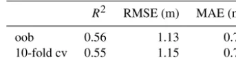
Table 2.Comparison of the RF generalization error quantified by the out-of-bag (oob) procedure and 10-fold cross-validation (cv) based on three metrics, i.e. coefficient of determination (R2) root-mean-squared error (RMSE) and mean absolute error (MAE). The 1900 additional observations were excluded for this evaluation.

R2 RMSE (m) MAE (m)

oob 0.56 1.13 0.76

10-fold cv 0.55 1.15 0.77

mean absolute error (MAE) and root-mean-squared error (RMSE), indicated an overall good performance (Table 2). More than half of the variance contained in the training data was captured by the RF model, the MAE amounted to 76 cm and the RMSE was 1.13 m. The density scatter plot in Fig. 3 zooms into the top 6 m, and it becomes apparent that very shallow observations (<0.5 m) were systematically biased while deeper observations were estimated in good agreement (close to the 1 : 1 line).

In order to investigate if the oob prediction is a reliable source to quantify how generalizable a RF model is, we con-ducted a 10-fold cross-validation (cv) test. For this test, the dataset was randomly split into 10 sets of approximately the same size. Then 10 RF models were trained on 90 % of the data so that each set was left out once and could be used for evaluation purposes. The cv results were strikingly similar to the oob prediction (Table 2). The agreement was convincing which qualified the oob prediction as an appropriate way to quantify the generalization error of our RF model.

Figure 3.The RF accuracy assessment was performed based on the out-of-bag sample technique. The axes depict the simulated (Sim) and observed (Obs) depth to the shallow water table. Panel(a)displays a standard scatter plot containing∼15 000 well data points. The 1900 additional observations are excluded. Panel(b)shows a zoom-in (extent indicators in red in panela) and the data are visualized as a density scatter plot. The colour bar represents the number of data points in each square.

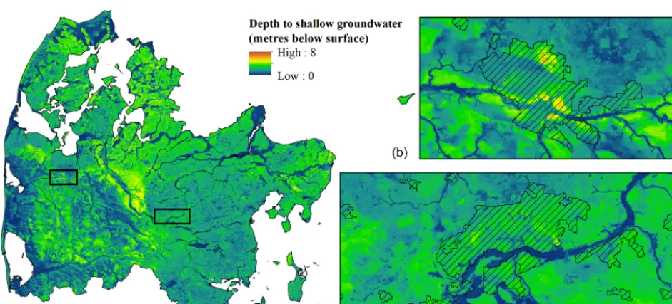
Figure 4.The resulting map of the depth to the shallow water table at a 50 m grid resolution. The zoomed-in extents highlight two urban areas. Panel(b)displays the city of Holstebro, and panel(c)depicts the city of Silkeborg. Urban areas are visualized using hatching.

3.2 Covariate sensitivity

Covariate sensitivity was analysed from two different per-spectives, both using the concept of permutation accuracy. First, sensitivity was assessed for the trained RF model based on the decrease in theR2of the oob prediction as a conse-quence of permuting a covariate. For this, only the training dataset was incorporated which resulted in an overall covari-ate sensitivity score. Second, the sensitivity of the trained RF model was estimated individually for each simulation grid based on the absolute difference between the permuted pre-diction and the original prepre-diction. This approach gives the relative ranking of the most sensitive covariates for each

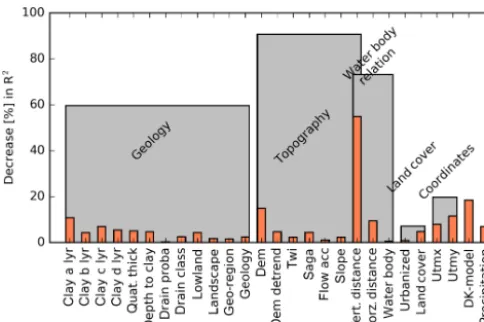
Figure 5.Variable importance of the trained RF model. The concept of permutation accuracy was implemented to quantify the decrease in out-of-bag performanceR2. Permutation was applied not only to single covariates (orange) but also to groups of covariates (grey). Covariates are further specified in Table 1.

depth to the shallow water table at a 500 m resolution for a 20-year reference period (1991–2010). This indicated that the DK-model could supply a valuable coarse trend to the RF model.

Figure 5 also quantifies the importance of physically re-lated covariates. When permuted collectively, covariates as-sociated with the topography resulted in a decrease of nearly 100 % in performance; thus, the respective covariates formed the most important group. They were followed by covariates describing the water body relation (∼70 % drop in perfor-mance) and geology-related variables (60 %). As the vertical distance to the nearest water body relates to both, topography and water body proximity, it was included in both groups. The above-mentioned results are based on the relative de-crease in theR2caused by the permutation of the covariates. In order to test if the resulting sensitivity ranking is metric dependent, we conducted the same analysis based on the rel-ative decrease in the RMSE. We concluded that, in spite of varying absolute numbers, the same conclusion in terms of relative covariate sensitivity could be drawn; therefore, the results are not discussed further in this study.

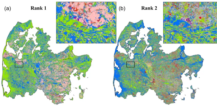
The results from the spatial sensitivity analyses are pre-sented in Fig. 6. Figure 6 depicts maps of the top two most important covariates for the RF prediction. Covariates were permuted collectively following the groups presented in Table 1 and as applied in the sensitivity analysis of the trained RF model (Fig. 5). Each covariate group was per-muted 250 times to ensure that the difference to the original RF prediction converged at the individual grids. The sim-ulated water table in the moraine landscape in the eastern part of the model domain was controlled by covariates re-lated to the geology. Here topography is gently undulating and sediments are clay rich, which, in combination, resulted in a water table close to the surface with small-scale

vari-ability caused by geological heterogeneity. The second-most important covariates in the moraine landscape were mainly the DK-model or the UTM coordinates. This underlined the complexity of the shallow water table in this landscape. The DK-model includes a comprehensive analysis of the entire system, taking the interplay between several factors (hydro-geology, topography, climate and others) into consideration. In the RF model, coordinates provided the only possibility to assign uniqueness to a simulation grid, which was required in the moraine landscape to capture the complexity of the shallow water table. Topography was important at locations close to sea level or areas that were generally plane. Water body relations played an important role at locations that were either very far away from or very close to a water body. Data on the location of urban areas, which were contained in the land cover group, were rated important for urban areas with moraine soils. In such clayey conditions, the subsurface is often drained resulting in a deeper water table. Overall, the importance of the DK-model appeared to be very local and generally scattered across the domain, which underlined the relevance of this covariate, as it could provide coarse infor-mation at locations where the standard covariates fail to pro-vide a meaningful generalization.

3.3 Uncertainty analysis

For the uncertainty analysis, we employed two methods, namely RFRK and QRF. For the first, the RF residuals were interpolated using kriging. Figure 7 shows the variogram model which was used in the kriging interpolation. The nugget was set to 0.26 m2and the sill was defined as 1.02 m2. An exponential variogram with a range of 700 m gave the most satisfying fit to the experimental semivariances calcu-lated at a 200 m lag distance.

Figure 6.The results of the sensitivity analysis are shown for the most sensitive covariate group (Rank 1,a) and the second-most important covariate group (Rank 2,b). The city of Holstebro is chosen as the zoomed-in region for both maps.

Figure 7.The computed semivariances for the RF residuals (cir-cles), based on the oob prediction. The line expresses the fitted var-iogram model.

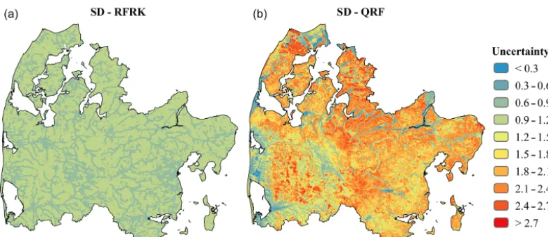
moraine landscape in the eastern part was characterized by an overall high uncertainty despite having an overall water table that is close to the surface. Such physical dependencies that relate to the structure of the RF model were not captured by the RFRK approach, which purely reflected borehole prox-imity. The mean uncertainty across the domain amounted to 0.92 m for RFRK and 1.68 m for QRF.

4 Discussion 4.1 Training dataset

Figure 8.Two methods to quantify the uncertainty of a RF model are implemented: RFRK(a)and QRF(b). For all maps, uncertainty is expressed as the standard deviation (SD).

In unconfined sandy aquifers, we assume the elevation of the shallow water table to be more homogeneous than the depth of the shallow water table. This assumption may not apply for more complex geological settings, such as glacial tills, which cover a majority of the study area, where a sec-ondary water table often follows the surface elevation. This motivated us to model the water table depth instead of the el-evation, which was further supported by an initial test where a RF model was trained to predict the water table elevation. The resulting water table elevation could easily be converted to depth via subtraction from the surface elevation, and re-sults indicated poorer performance compared with the RF model predicting the water table depth.

The RF model was trained to a single event and thus dis-regards the temporal dynamics of the shallow groundwater system. As the model was designed as a simple screening tool, this can be considered an advantage; however, much of the complexity is not considered which is a clear shortcom-ing of the proposed method.

In the coming years, the Danish national water resources model (DK-model) will be updated based on recent hydro-geological interpretations and reconstructed at a 100 m spa-tial resolution. This is expected to improve the predictability of the shallow water table, and the DK-model output should then be utilized to update the RF model.

4.2 Random forests model

This study utilized the oob prediction to validate the per-formance of the RF model based on three metrics, namely the coefficient of determination (R2), mean absolute error (MAE) and root-mean-squared error (RMSE). The metric scores were very satisfying overall and in the range of what could be considered very acceptable in groundwater flow modelling (Henriksen et al., 2003). These findings underpin the applicability of RF to model complex, non-linear

vari-ables with an accuracy that is difficult to obtain with physi-cally based models. In contrast, the accuracy assessment re-vealed a systematic bias of the trained RF model that was af-fecting wells with groundwater levels close to the terrain. The biased wells were predominately located in clayey moraine sediments, which indicated location-specific shortcomings of the RF model. The geology of the moraine landscape is het-erogeneous which impacts the hydrogeological setting and, in turn, also the shallow groundwater (He et al., 2014, 2015). At the current stage, the available national hydrogeological data do not possess the required spatial resolution to resolve the apparent heterogeneities adequately. Moreover, some of the above-mentioned wells are placed in confined conditions, which in combination with the heterogeneous geology may hinder good performance of the RF model.

Studying the covariate importance identified the water ta-ble simulated with the DK-model at a 500 m resolution as the second-most important RF input. These results were very promising as the applied RF framework forms a straightfor-ward implementation of unifying machine learning and phys-ically based models. More precisely, RF built upon the coarse DK-model using high-resolution covariate information that ensured physical consistency.

The resulting spatial resolution of 50 m provides a valu-able screening tool for water management purposes. The risk of groundwater floods on agricultural fields or urban areas is typically very local and driven by small-scale variations of topography and geology. This makes high-resolution predic-tions inevitable in order to reliably tackle the related chal-lenges. At the regional scale, the 50 m resolution would not be feasible with numerical modelling, which emphasizes the versatile applicability of RF. Many covariates are available at a finer resolution and, as computational power becomes more and more dispensable, RF predictions at even higher resolution are within reach. This development should also build upon current improvements of physically based mod-els, which are now already capable of providing results at resolutions in the range of hundreds of metres (Ko et al., 2019; Wood et al., 2011) and, thus, such models could pro-vide valuable trends, used as covariates in machine learning models.

This study proposed a novel approach to quantify the co-variate sensitivity of the simulation dataset, which results in a relative ranking of the most important covariates at the grid level. This analysis provided physical insights into the driv-ing mechanisms and, in general, the finddriv-ings corresponded to the conceptual understanding of the hydrogeology in the study area. Such sensitivity maps are extremely valuable for both the modeller and the stakeholders working with RF pre-dictions. The former group can validate the physical consis-tency of the otherwise nontransparent black-box model and the latter will have a better understanding and ultimately also a greater acceptance of the predictions.

4.3 Uncertainty assessment

This study assessed the capabilities of RFRK and QRF to es-timate the uncertainties associated with a RF model that pre-dicts water levels of the shallow groundwater system. Uncer-tainty was expressed by the standard deviation; alternatively, both methods could also be utilized to map upper and lower uncertainty bounds that represent certain confidence inter-vals. The key differences between the two proposed methods were as follows: (1) the uncertainty estimation of RFRK was generally lower than QRF and (2) the spatial patterns were diverging; RFRK only reflected borehole proximity, whereas QRF manifested a physical dependency of the uncertainty estimation. These findings are in line with recent compari-son studies focusing on QRF and RFRK from the digital soil mapping literature (Szatmári and Pásztor, 2018; Vaysse and Lagacherie, 2017). Szatmári and Pásztor (2018) argue that RFRK-based uncertainty estimations are limited because re-sults do not depend on the data value; therefore, the method expresses an unconditional variance. This stringent assump-tion of homoscedasticity, i.e. constant error variance, could be unrealistic for variables where the variance behaves pro-portionally to the measured value (Hengl et al., 2018). More-over, RFRK assumes that the RF prediction, which is used

as a trend, is certain; thus, the kriging variance only reflects the distance to the nearest observation. This assumption is too optimistic, as the uncertainty in the RF prediction is ne-glected. Once the training dataset is processed, RF disre-gards any uncertainties associated with the values of the tar-get variable. In this study, uncertainties could originate from the applied sinus model used to transfer the observations to a typical wintertime minimum depth as well as the obser-vations itself. In contrast, a physically based hydrological model allows more transparency, as biased observations will be marked as outliers in the model evaluation. However, a data-driven model, as flexible as RF, will incorporate such outliers – thus biased predictions may arise.

As stated by Vaysse and Lagacherie (2017), QRF quanti-fies information regarding where a simulation point is located in the covariate space. In this way, QRF properly discrim-inates groundwater conditions of contrasted physical com-plexities, of which some are better constrained by the train-ing dataset than others. We argue that the RFRK shortcom-ings of assuming certainty in the trend prediction can be al-leviated by the addition of QRF, which can capture the un-certainty of the RF model structure. In summary, RFRK cap-tures uncertainty related to the geographical space, whereas QRF describes uncertainties related to the covariate space. More work is needed to integrate these two sources of uncer-tainty into a single unceruncer-tainty quantification.

Reducing uncertainties can be achieved by collecting more observations and, thus, expanding the training dataset. Es-pecially in the eastern part of the domain, which is char-acterized by a high clay content and a heterogeneous sur-ficial geology, additional data would likely reduce the un-certainty. A measuring campaign in wintertime, when the shallow groundwater system is fully replenished, would be very beneficial to advancing the modelling capabilities. Ad-ditionally, a higher spatial resolution may contribute to an un-certainty reduction, as observations can be represented more uniquely by the covariates.

In more general terms, as the numbers of hydrological ap-plications based on machine learning are vastly expanding, standards on how to conduct uncertainty analyses must be formalized in the same fashion as was carried out for numer-ical modelling (Refsgaard et al., 2007). Ultimately, such a development determines the stakeholder acceptance of ma-chine learning results.

5 Conclusions

valuable for water resources management. We draw the fol-lowing main conclusions from our work:

1. RF is a versatile modelling tool with high accuracy that enables spatial detail beyond the possibilities of (physi-cally based) numerical modelling. The depth to the shal-low water table was modelled with a mean absolute er-ror of 76 cm for an independent evaluation test. 2. Predictions from a coarse physically based model that

represent an overall trend of the water table can be uti-lized by RF as a covariate. In this way, RF ensures physical consistency at coarse scale and exhausts high-resolution information from topography, geology and other relevant variables. The DK-model at 500 m res-olution was rated the second-most important covariate in the trained RF model, indicating that this simple form of unifying machine learning and physically based mod-elling has great potential.

3. The novel approach to assess covariate sensitivity for the prediction dataset goes beyond the standard applica-tions where covariate importance is solely quantified for the training dataset. Results provide valuable insights on the spatial pattern of covariate sensitivity and can contribute to generating acceptability among end-users. The increased interpretability of the RF predictions can reassure modellers by comparing the derived sensitiv-ity patterns with their conceptual understanding of the system.

4. In the general context of hydrological machine learning applications, more experience must be gained on how to properly quantify uncertainty. RFRK was found use-ful to assess observational proximity, but assuming cer-tainty in the RF predications was regarded a shortcom-ing. This can be compensated for by QRF, which is ca-pable of addressing the uncertainty related to the struc-ture of the RF model. However, methods to remove the uncertainties related to the observations themselves and possible preprocessing of the training dataset are still lacking.

Code and data availability. The covariate data used to conduct this study are available upon request from the corresponding author (Julian Koch). The raw water level observations are freely available on the Jupiter database (http://data.geus.dk/geusmap/?mapname= jupiter&lang=en\#baslay=baseMapDa&optlay=&extent=-213120, 5884060,1323130,6565940, last access: January 2019; Hansen and Pjetursson, 2011), and the processed minimum values are available upon request. All code is available upon request from the corresponding author.

Author contributions. JK designed and executed the modelling work, lead the data analysis and wrote the initial draft of the paper.

HB compiled the training dataset. HJH and TOS contributed scien-tifically to the modelling and data analysis. All authors contributed to the paper by providing comments and suggestions.

Competing interests. The authors declare that they have no conflict of interest.

Acknowledgements. The work has been carried out with financial support granted by the Coast to Coast Climate Challenge project funded by the EU’s LIFE programme.

Financial support. This research has been supported by the EU LIFE (grant no. LIFE15 IPC/DK/000006).

Review statement. This paper was edited by Graham Fogg and re-viewed by Anders Bjørn Møller and Katherine Ransom.

References

Adhikari, K., Kheir, R. B., Greve, M. B., Bøcher, P. K., Malone, B. P., Minasny, B., McBratney, A. B., and Greve, M. H.: High-Resolution 3-D Mapping of Soil Texture in Denmark, Soil Sci. Soc. Am. J., 9, e105519, https://doi.org/10.2136/sssaj2012.0275, 2013.

Adhikari, K., Hartemink, A. E., Minasny, B., Bou Kheir, R., Greve, M. B., and Greve, M. H.: Digital Mapping of Soil Organic Car-bon Contents and Stocks in Denmark, PLoS One, 9, e105519, https://doi.org/10.1371/journal.pone.0105519, 2014.

Ahmed, Z. U., Woodbury, P. B., Sanderman, J., Hawke, B., Jauss, V., Solomon, D., and Lehmann, J.: Assessing soil carbon vul-nerability in the Western USA by geospatial modeling of pyro-genic and particulate carbon stocks, J. Geophys. Res.-Biogeo., 122, 354–369, https://doi.org/10.1002/2016JG003488, 2017. Asher, M. J., Croke, B. F. W., Jakeman, A. J., and Peeters, L.

J. M.: A review of surrogate models and their application to groundwater modeling, Water Resour. Res., 51, 5957–597, https://doi.org/10.1002/2015WR016967, 2015.

Banerjee, P., Prasad, R. K., and Singh, V. S.: Forecasting of ground-water level in hard rock region using artificial neural network, Environ. Geol., 58, 1239–1246, https://doi.org/10.1007/s00254-008-1619-z, 2009.

Best, M. J., Abramowitz, G., Johnson, H. R., Pitman, A. J., Bal-samo, G., Boone, A., Cuntz, M., Decharme, B., Dirmeyer, P. A., Dong, J., Ek, M., Guo, Z., Haverd, V., van den Hurk, B. J. J., Nearing, G. S., Pak, B., Peters-Lidard, C., Santanello, J. A., Stevens, L., and Vuichard, N.: The Plumbing of Land Surface Models: Benchmarking Model Performance, J. Hydrometeo-rol., 16, 1425–1442, https://doi.org/10.1175/JHM-D-14-0158.1, 2015.

Biau, G. and Scornet, E.: A random forest guided tour, Test, 25, 197–227, https://doi.org/10.1007/s11749-016-0481-7, 2016. Binzer, K. and Stockmarr, J.: Geological map of Denmark

1 : 500 000 (pre-quaternary surface topography of Denmark). Mapseries – DGU, Danmarks Geologiske Undersøgelse, 1994. Böhner, J. and Selige, T.: Spatial prediction of soil attributes

us-ing terrain analysis and climate regionalisation, Göttus-inger Geogr. Abhandlungen, SAGA – Analysis and Modelling Applications, 115, 13–28, 2002.

Breiman, L.: Random forests, Mach. Learn., 45, 5–32, https://doi.org/10.1023/A:1010933404324, 2001.

Breuning-Madsen, H. and Jensen, N. H.: Pedological Regional Vari-ations in Well-drained Soils, Denmark, Geogr. Tidsskr. J. Geogr., 92, 61–69, https://doi.org/10.1080/00167223.1992.10649316, 1992.

Bricker, S. H., Banks, V. J., Galik, G., Tapete, D., and Jones, R.: Ac-counting for groundwater in future city visions, Land Use Policy, 69, 618–630, https://doi.org/10.1016/j.landusepol.2017.09.018, 2017.

Chaney, N. W., Van Huijgevoort, M. H. J., Shevliakova, E., Maly-shev, S., Milly, P. C. D., Gauthier, P. P. G., and Sulman, B. N.: Harnessing big data to rethink land heterogeneity in Earth system models, Hydrol. Earth Syst. Sci., 22, 3311–3330, https://doi.org/10.5194/hess-22-3311-2018, 2018.

Clayton, D. and Andre, J.: GSLIB – Geostatistical software library and user’s guide, Technometrics, 119, p. 147, 1998.

Close, M. E., Abraham, P., Humphries, B., Lilburne, L., Cuthill, T., and Wilson, S.: Predicting groundwater redox status on a regional scale using linear discriminant analysis, J. Contam. Hydrol., 191, 19–32, https://doi.org/10.1016/j.jconhyd.2016.04.006, 2016. Daliakopoulos, I. N., Coulibaly, P., and Tsanis, I. K.: Groundwater

level forecasting using artificial neural networks, J. Hydrol., 309, 229–240, https://doi.org/10.1016/j.jhydrol.2004.12.001, 2005. Erickson, M. L., Elliott, S. M., Christenson, C. A., and Krall,

A. L.: Predicting geogenic Arsenic in Drinking Water Wells in Glacial Aquifers, North-Central USA: Accounting for Depth-Dependent Features, Water Resour. Res., 54, 10–172, https://doi.org/10.1029/2018WR023106, 2018.

Fallah-Mehdipour, E., Bozorg Haddad, O., and Mariño, M. A.: Prediction and simulation of monthly groundwater levels by genetic programming, J. Hydro-Environ. Res., 7, 253–260, https://doi.org/10.1016/j.jher.2013.03.005, 2013.

Fan, Y., Li, H., and Miguez-Macho, G.: Global patterns of groundwater table depth, Science, 339, 940–943, https://doi.org/10.1126/science.1229881, 2013.

Ferguson, I. M. and Maxwell, R. M.: Role of groundwa-ter in watershed response and land surface feedbacks under climate change, Water Resour. Res., 46, 1–15, https://doi.org/10.1029/2009WR008616, 2010.

Fienen, M. N., Masterson, J. P., Plant, N. G., Gutierrez, B. T., and Thieler, E. R.: Bridging groundwater models and decision sup-port with a Bayesian network, Water Resour. Res., 49, 6459– 6473, https://doi.org/10.1002/wrcr.20496, 2013.

Francke, T., López-Tarazón, J. A., and Schröder, B.: Estimation of suspended sediment concentration and yield using linear models, random forests and quantile regression forests, Hydrol. Process., 22, 4892–4904, https://doi.org/10.1002/hyp.7110, 2008. Gleeson, T., Befus, K. M., Jasechko, S., Luijendijk, E.,

and Cardenas, M. B.: The global volume and

distribu-tion of modern groundwater, Nat. Geosci., 9, 161–167, https://doi.org/10.1038/ngeo2590, 2016.

Guo, P. T., Li, M. F., Luo, W., Tang, Q. F., Liu, Z. W., and Lin, Z. M.: Digital mapping of soil organic matter for rub-ber plantation at regional scale: An application of random for-est plus residuals kriging approach, Geoderma, 237–238, 49–59, https://doi.org/10.1016/j.geoderma.2014.08.009, 2015.

Hansen, M. and Pjetursson, B.: Free, online Danish shallow geolog-ical data, Geol. Surv. Denmark Greenl. Bull., 23, 53–56, 2011. He, X., Koch, J., Sonnenborg, T. O., Jørgensen, F.,

Scham-per, C., and Christian Refsgaard, J.: Transition probability-based stochastic geological modeling using airborne geophysi-cal data and borehole data, Water Resour. Res., 50, 3147–3169, https://doi.org/10.1002/2013WR014593, 2014.

He, X., Højberg, A. L., Jørgensen, F., and Refsgaard, J. C.: As-sessing hydrological model predictive uncertainty using stochas-tically generated geological models, Hydrol. Process., 29, 4293– 4311, https://doi.org/10.1002/hyp.10488, 2015.

Hengl, T., Heuvelink, G. B. M., and Rossiter, D. G.: About regression-kriging: From equations to case studies, Comput. Geosci., 33, 1301–1315, https://doi.org/10.1016/j.cageo.2007.05.001, 2007.

Hengl, T., Heuvelink, G. B. M., Kempen, B., Leenaars, J. G. B., Walsh, M. G., Shepherd, K. D., Sila, A., MacMillan, R. A., De Jesus, J. M., Tamene, L., and Tondoh, J. E.: Mapping soil properties of Africa at 250 m resolution: Random forests signif-icantly improve current predictions, PLoS One, 10, e0125814, https://doi.org/10.1371/journal.pone.0125814, 2015.

Hengl, T., Nussbaum, M., Wright, M. N., Heuvelink, G. B. M., and Gräler, B.: Random forest as a generic framework for predic-tive modeling of spatial and spatio-temporal variables, PeerJ, 6, e5518, https://doi.org/10.7717/peerj.5518, 2018.

Henriksen, H. J., Troldborg, L., Nyegaard, P., Sonnenborg, T. O., Refsgaard, J. C., and Madsen, B.: Methodology for construction, calibration and validation of a national hydrological model for Denmark, J. Hydrol., 280, 52–71, https://doi.org/10.1016/S0022-1694(03)00186-0, 2003.

Henriksen, H. J., Troldborg, L., Højberg, A. L., and Refsgaard, J. C.: Assessment of exploitable groundwater resources of Den-mark by use of ensemble resource indicators and a numeri-cal groundwater–surface water model, J. Hydrol., 348, 224–240, 2008.

Henriksen, H. J., Højberg, A. . L., Olsen, M., Seaby, L. P., van der Keur, P., Stisen, S., Troldborg, L., Sonnenborg, T. O., and Ref-sgaard, J. C.: Klimaeffekter på hydrologi og grundvand (Klima-grundvandskort), Geological Survey of Denmark and Greenland, Copenhagen Denmark, 1–116, 2012 (in Danish).

Højberg, A. L., Troldborg, L., Stisen, S., Christensen, B. B. S., and Henriksen, H. J.: Stakeholder driven update and improvement of a national water resources model, Environ. Model. Softw., 40, 202–213, https://doi.org/10.1016/j.envsoft.2012.09.010, 2013. Jankowfsky, S., Branger, F., Braud, I., Rodriguez, F., Debionne,

S., and Viallet, P.: Assessing anthropogenic influence on the hydrology of small peri-urban catchments: Development of the object-oriented PUMMA model by integrating urban and rural hydrological models, J. Hydrol., 517, 1056–1071, https://doi.org/10.1016/j.jhydrol.2014.06.034, 2014.

require-ments and crop yields, Agr. Water Manage., 76, 24–35, https://doi.org/10.1016/j.agwat.2005.01.005, 2005.

Karlsson, I. B., Sonnenborg, T. O., Refsgaard, J. C., Trolle, D., Børgesen, C. D., Olesen, J. E., Jeppesen, E., and Jensen, K. H.: Combined effects of climate models, logical model structures and land use scenarios on hydro-logical impacts of climate change, J. Hydrol., 535, 301–317, https://doi.org/10.1016/j.jhydrol.2016.01.069, 2016.

Karpatne, A., Atluri, G., Faghmous, J. H., Steinbach, M., Baner-jee, A., Ganguly, A., Shekhar, S., Samatova, N., and Kumar, V.: Theory-guided data science: A new paradigm for scientific discovery from data, IEEE T. Knowl. Data En., 29, 2318–2331, https://doi.org/10.1109/TKDE.2017.2720168, 2017.

Kidmose, J., Refsgaard, J. C., Troldborg, L., Seaby, L. P., and Es-crivà, M. M.: Climate change impact on groundwater levels: en-semble modelling of extreme values, Hydrol. Earth Syst. Sci., 17, 1619–1634, https://doi.org/10.5194/hess-17-1619-2013, 2013. Ko, A., Mascaro, G., and Vivoni, E. R.: Strategies to Improve

and Evaluate Physics-Based Hyperresolution Hydrologic Simu-lations at Regional Basin Scales, Water Resour. Res., 55, 1129– 1152, https://doi.org/10.1029/2018WR023521, 2019.

Koch, J., Stisen, S., Refsgaard, J. C., Ernstsen, V., Jakobsen, P. R., and Højberg, A. L.: Modeling Depth of the Redox Interface at High Resolution at National Scale Using Random Forest and Residual Gaussian Simulation, Water Resour. Res., 55, 1451– 1469, https://doi.org/10.1029/2018WR023939, 2019.

Kollet, S. J. and Maxwell, R. M.: Capturing the influence of ground-water dynamics on land surface processes using an integrated, distributed watershed model, Water Resour. Res., 44, W02402, https://doi.org/10.1029/2007WR006004, 2008.

Kreibich, H. and Thieken, A. H.: Assessment of damage caused by high groundwater inundation, Water Resour. Res., 44, W09409, https://doi.org/10.1029/2007WR006621, 2008.

Larsen, M. A. D., Christensen, J. H., Drews, M., Butts, M. B., and Refsgaard, J. C.: Local control on precipitation in a fully coupled climate-hydrology model, Sci. Rep., 6, 22927, https://doi.org/10.1038/srep22927, 2016.

Li, J., Heap, A. D., Potter, A., and Daniell, J. J.: Application of machine learning methods to spatial interpolation of envi-ronmental variables, Environ. Model. Softw., 26, 1647–1659, https://doi.org/10.1016/j.envsoft.2011.07.004, 2011.

Ließ, M., Glaser, B., and Huwe, B.: Uncertainty in the spa-tial prediction of soil texture. Comparison of regression tree and Random Forest models, Geoderma, 170, 70–79, https://doi.org/10.1016/j.geoderma.2011.10.010, 2012.

Lutz, S. R., Krieg, R., Müller, C., Zink, M., Knöller, K., Samaniego, L., and Merz, R.: Spatial Patterns of Water Age: Using Young Water Fractions to Improve the Characterization of Transit Times in Contrasting Catchments, Water Resour. Res., 54, 4767–4784, https://doi.org/10.1029/2017WR022216, 2018.

MacDonald, A., Hughes, A., Adams, B., Bloomfield, J., McKenzie, A., and Macdonald, D.: Improving the understanding of the risk from groundwater flooding in the UK, in: FLOODrisk 2008, Eu-ropean Conference on Flood Risk Management, 30 September– 2 October 2008, Oxford, UK, CRC Press, 2010.

MacDonald, D., Dixon, A., Newell, A., and Hallaways, A.: Groundwater flooding within an urbanised flood plain, J. Flood Risk Manag., 5, 68–80, https://doi.org/10.1111/j.1753-318X.2011.01127.x, 2012.

Matheron, G.: Principles of geostatistics, Econ. Geol., 58, 1246– 1266, https://doi.org/10.2113/gsecongeo.58.8.1246, 1963. Maxwell, R. M. and Condon, L. E.: Connections between

ground-water flow and transpiration partitioning, Science, 353, 377–380, https://doi.org/10.1126/science.aaf7891, 2016.

Meinshausen, N.: Quantile Regression Forests, J. Mach. Learn. Res., 7, 983–999, https://doi.org/10.1111/j.1541-0420.2010.01521.x, 2006.

Møller, A. B., Iversen, B. V., Beucher, A., and Greve, M. H.: Prediction of soil drainage classes in Denmark by means of decision tree classification, Geoderma, 352, 314–329, https://doi.org/10.1016/j.geoderma.2017.10.015, 2017.

Møller, A. B., Beucher, A., Iversen, B. V., and Greve, M. H.: Predicting artificially drained areas by means of a selective model ensemble, Geoderma, 320, 30–42, https://doi.org/10.1016/j.geoderma.2018.01.018, 2018.

Mutanga, O., Adam, E., and Cho, M. A.: High density biomass estimation for wetland vegetation using worldview-2 imagery and random forest regression algorithm, Int. J. Appl. Earth Obs. Geoinf., 18, 399–406, https://doi.org/10.1016/j.jag.2012.03.012, 2012.

Nearing, G. S., Mocko, D. M., Peters-Lidard, C. D., Kumar, S. V., and Xia, Y.: Benchmarking NLDAS-2 Soil Moisture and Evapo-transpiration to Separate Uncertainty Contributions, J. Hydrome-teorol., 17, 745–759, https://doi.org/10.1175/JHM-D-15-0063.1, 2016.

Nolan, B. T., Fienen, M. N., and Lorenz, D. L.: A statisti-cal learning framework for groundwater nitrate models of the Central Valley, California, USA, J. Hydrol., 531, 902–911, https://doi.org/10.1016/j.jhydrol.2015.10.025, 2015.

Nussbaum, M., Spiess, K., Baltensweiler, A., Grob, U., Keller, A., Greiner, L., Schaepman, M. E., and Papritz, A.: Evaluation of digital soil mapping approaches with large sets of environmental covariates, SOIL, 4, 1–22, https://doi.org/10.5194/soil-4-1-2018, 2018.

Odeh, I. O. A., McBratney, A. B., and Chittleborough, D. J.: Further results on prediction of soil properties from terrain attributes: het-erotopic cokriging and regression-kriging, Geoderma, 67, 215– 226, https://doi.org/10.1016/0016-7061(95)00007-B, 1995. Pebesma, E. J.: Multivariable geostatistics in S: The

gstat package, Comput. Geosci., 30, 683–691, https://doi.org/10.1016/j.cageo.2004.03.012, 2004.

Pedregosa, F., Varoquaux, G., Gramfort, A., Michel, V., Thirion, B., Grisel, O., Blondel, M., Prettenhofer, P., Weiss, R., Dubourg, V., Vanderplas, J., Passos, A., Cournapeau, D., Brucher, M., Per-rot, M., and Duchesnay, É.: Scikit-learn: Machine Learning in Python, J. Mach. Learn. Res., 12, 2825–2830, 2012.

Refsgaard, J. C., van der Sluijs, J. P., Højberg, A. L., and Vanrol-leghem, P. A.: Uncertainty in the environmental modelling pro-cess – A framework and guidance, Environ. Model. Softw., 22, 1543–1556, https://doi.org/10.1016/j.envsoft.2007.02.004, 2007. Reichstein, M., Camps-Valls, G., Stevens, B., Jung, M., Denzler, J., Carvalhais, N., and Prabhat: Deep learning and process un-derstanding for data-driven Earth system science, Nature, 566, 195–204, https://doi.org/10.1038/s41586-019-0912-1, 2019. Richey, A. S., Thomas, B. F., Lo, M. H., Famiglietti, J. S., Swenson,

Res., 51, 5198–5216, https://doi.org/10.1002/2015WR017351, 2015.

Rodell, M., Famiglietti, J. S., Wiese, D. N., Reager, J. T., Beau-doing, H. K., Landerer, F. W., and Lo, M. H.: Emerging trends in global freshwater availability, Nature, 557, 651–659, https://doi.org/10.1038/s41586-018-0123-1, 2018.

Rodriguez-Galiano, V., Mendes, M. P., Garcia-Soldado, M. J., Chica-Olmo, M., and Ribeiro, L.: Predictive model-ing of groundwater nitrate pollution usmodel-ing Random For-est and multisource variables related to intrinsic and spe-cific vulnerability: A case study in an agricultural setting (Southern Spain), Sci. Total Environ., 476–477, 189–206, https://doi.org/10.1016/j.scitotenv.2014.01.001, 2014.

Rodriguez-Galiano, V., Sanchez-Castillo, M., Chica-Olmo, M., and Chica-Rivas, M.: Machine learning predictive models for mineral prospectivity: An evaluation of neural networks, random forest, regression trees and support vector machines, Ore Geol. Rev., 71, 804–818, https://doi.org/10.1016/j.oregeorev.2015.01.001, 2015. Shen, C., Laloy, E., Elshorbagy, A., Albert, A., Bales, J., Chang, F.-J., Ganguly, S., Hsu, K.-L., Kifer, D., Fang, Z., Fang, K., Li, D., Li, X., and Tsai, W.-P.: HESS Opinions: In-cubating deep-learning-powered hydrologic science advances as a community, Hydrol. Earth Syst. Sci., 22, 5639–5656, https://doi.org/10.5194/hess-22-5639-2018, 2018.

Shiri, J., Kisi, O., Yoon, H., Lee, K. K., and Hossein Nazemi, A.: Predicting groundwater level fluctuations with mete-orological effect implications-A comparative study among soft computing techniques, Comput. Geosci., 56, 32–44, https://doi.org/10.1016/j.cageo.2013.01.007, 2013.

Stisen, S., Sonnenborg, T. O., Refsgaard, J. C., Koch, J., Bircher, S., and Jensen, K. H.: Moving beyond runoff calibration – Multi-constraint optimization of a surface-subsurface-atmosphere model, Hydrol. Process., 32, 2654–2668, https://doi.org/10.1002/hyp.13177, 2018.

Szatmári, G. and Pásztor, L.: Comparison of various un-certainty modelling approaches based on geostatistics and machine learning algorithms, Geoderma, 337, 1329–1340, https://doi.org/10.1016/J.GEODERMA.2018.09.008, 2018. Tesoriero, A. J., Terziotti, S., and Abrams, D. B.:

Pre-dicting Redox Conditions in Groundwater at a Re-gional Scale, Environ. Sci. Technol., 49, 9657–9664, https://doi.org/10.1021/acs.est.5b01869, 2015.

Tesoriero, A. J., Gronberg, J. A., Juckem, P. F., Miller, M. P., and Austin, B. P.: Predicting redox-sensitive con-taminant concentrations in groundwater using random forest classification, Water Resour. Res., 53, 7316–7331, https://doi.org/10.1002/2016WR020197, 2017.

Upton, K. A. and Jackson, C. R.: Simulation of the spatio-temporal extent of groundwater flooding using statistical methods of hydrograph classification and lumped parameter models, Hy-drol. Process., 25, 1949–1963, https://doi.org/10.1002/hyp.7951, 2011.

van Roosmalen, L., Christensen, B. S. B., and Sonnenborg, T. O.: Regional Differences in Climate Change Impacts on Groundwa-ter and Stream Discharge in Denmark, Vadose Zone J., 6, 554– 571, https://doi.org/10.2136/vzj2006.0093, 2007.

Vaysse, K. and Lagacherie, P.: Using quantile regression forest to estimate uncertainty of digital soil mapping products, Geoderma, 291, 55–64, https://doi.org/10.1016/j.geoderma.2016.12.017, 2017.

Viscarra Rossel, R. A., Webster, R., and Kidd, D.: Mapping gamma radiation and its uncertainty from weathering prod-ucts in a Tasmanian landscape with a proximal sensor and random forest kriging, Earth Surf. Proc. Land., 39, 735–748, https://doi.org/10.1002/esp.3476, 2014.

Wang, F., Ducharne, A., Cheruy, F., Lo, M.-H., and Grandpeix, J.-Y.: Impact of a shallow groundwater table on the global water cycle in the IPSL land–atmosphere coupled model, Clim. Dy-nam., 50, 3505–3522, https://doi.org/10.1007/s00382-017-3820-9, 2018.

Winkel, L. H. E., Trang, P. T. K., Lan, V. M., Stengel, C., Amini, M., Ha, N. T., Viet, P. H., and Berg, M.: Arsenic pollution of ground-water in Vietnam exacerbated by deep aquifer exploitation for more than a century, P. Natl. Acad. Sci. USA, 108, 1246–1251, https://doi.org/10.1073/PNAS.1011915108, 2011.

Wood, E. F., Roundy, J. K., Troy, T. J., Van Beek, L. P. H., Bierkens, M. F. P., Blyth, E., de Roo, A., Döll, P., Ek, M., and Famigli-etti, J.: Hyperresolution global land surface modeling: Meeting a grand challenge for monitoring Earth’s terrestrial water, Water Resour. Res., 47, 1–10, 2011.

Yoon, H., Jun, S. C., Hyun, Y., Bae, G. O., and Lee, K. K.: A comparative study of artificial neural networks and support vector machines for predicting groundwater levels in a coastal aquifer, J. Hydrol., 396, 128–138, https://doi.org/10.1016/j.jhydrol.2010.11.002, 2011.

Youssef, A. M., Pourghasemi, H. R., Pourtaghi, Z. S., and Al-Katheeri, M. M.: Landslide susceptibility mapping using random forest, boosted regression tree, classification and regression tree, and general linear models and comparison of their performance at Wadi Tayyah Basin, Asir Region, Saudi Arabia, Landslides, 13, 839–856, https://doi.org/10.1007/s10346-015-0614-1, 2016. Zimmermann, B., Zimmermann, A., Turner, B. L., Francke, T., and Elsenbeer, H.: Connectivity of overland flow by drainage net-work expansion in a rain forest catchment, Water Resour. Res., 50, 1457–1473, https://doi.org/10.1002/2012WR012660, 2014. Zipper, S. C., Soylu, M. E., Booth, E. G., and Loheide, S. P.: