Positive Impact Program Evaluation

ScholarWorks @ Georgia State University

ScholarWorks @ Georgia State University

Geosciences Theses Department of Geosciences

Fall 8-15-2012

Caprock Interactions with the Supercritical CO2 and Brine: A

Caprock Interactions with the Supercritical CO2 and Brine: A

Labratory Study of the Effects of Simulated Geological CO2

Labratory Study of the Effects of Simulated Geological CO2

Sequestration on Shales from the Black Warrior River Basin,

Sequestration on Shales from the Black Warrior River Basin,

Alabama L

Alabama L

Jessica E. Raines

Follow this and additional works at: https://scholarworks.gsu.edu/geosciences_theses

Recommended Citation Recommended Citation

Raines, Jessica E., "Caprock Interactions with the Supercritical CO2 and Brine: A Labratory Study of the Effects of Simulated Geological CO2 Sequestration on Shales from the Black Warrior River Basin, Alabama L." Thesis, Georgia State University, 2012.

https://scholarworks.gsu.edu/geosciences_theses/50

OF SIMULATED GEOLOGICAL CO2 SEQUESTRATION ON SHALES FROM THE BLACK WARRIOR RIVER BASIN, ALABAMA

by

JESSICA RAINES

Under the Direction of Daniel M. Deocampo ABSTRACT

A better understanding of the brine-rock- supercritical CO2 interaction is needed to evaluate the risks of geologic CO2 sequestration. The geochemical effects of brine and supercritical CO2 were exam-ined via laboratory modeling of in situ conditions on two reservoir caprocks in the Black Warrior River Basin, the Pottsville and Parkwood Formations. The clay fraction was extracted and treated at ~ 100 bar and 363 K (90 °C) over periods of up to 70 hours. Supercritical CO2 was introduced as dry ice in a pres-surized vessel. Samples were observed using XRD, WD-XRF, AA, SEM, and EDS. Clay fractions contained Fe-chlorite, illite, kaolinite, and quartz. Results show the dissolution of illite, CO2-brine induced cation exchange ok K+, and the dissolution of silicate minerals. Steady-state K/Si ratios in the fluid suggest quartz re-precipitation. These interactions could adversely affect the long-term storativity of the caprock and point to a need for further study.

OF SIMULATED GEOLOGICAL CO2 SEQUESTRATION ON SHALES FROM THE BLACK WARRIOR RIVER BASIN, ALABAMA

by

JESSICA RAINES

A Thesis Submitted in Partial Fulfillment of the Requirements for the Degree of Master of Science

in the College of Arts and Sciences Georgia State University

Copyright by Jessica Elizabeth Raines

OF SIMULATED GEOLOGICAL CO2 SEQUESTRATION ON SHALES FROM THE BLACK WARRIOR RIVER BASIN, ALABAMA

by

JESSICA RAINES

Committee Chair: Daniel M. Deocampo

Committee: Seth E. Rose

W. Crawford Elliott

Electronic Version Approved:

DEDICATION

ACKNOWLEDGEMENTS

I would like to acknowledge all those that helped me along the way. I would like to thank Frank Williams, my favorite anthropology professor, for being the first professor to show confidence in my abilities. Your passion directly influenced my educational experience and taught me to love research. To Seth Rose, my first geology professor, you sparked the fire that eventually led me to a Master of Sci-ence in Geology, and your classes continue to be the cornerstone of my educational experiSci-ence. Ken Terrell, without your advice, I would never have pursued geology. Thank you. Dan Deocampo, thank you for your immeasurable patience and time. Your guidance directly influenced the outcome of this document. Crawford Elliott, thank you for pushing me to continue my education and pursue a Master’s degree.

TABLE OF CONTENTS

ACKNOWLEDGEMENTS ... v

LIST OF EQUATIONS ... xii

1 INTRODUCTION ...1

1.1 Overview ...1

1.2 Carbon Sequestration ...6

1.2.1 Carbon Dioxide ...7

1.2.2 Carbon Storage ...7

1.3 Purpose of the Study ...8

1.4 Previous Research ... 10

1.5 Geological Setting ... 13

1.5.1 Black Warrior Basin ... 13

1.5.1.1 Pottsville Formation ... 15

1.5.1.2 Parkwood Formation ... 15

1.5.2 Sample Location ... 16

2 EXPERIMENT ... 17

2.1 Procedural Overview ... 17

2.2 Sample Analysis Methods ... 18

2.2.1 Thin Section Preparation... 18

2.2.3 XRF Analysis ... 22

2.2.3.1 XRF Data Treatment ... 23

2.2.4 AA Analysis ... 24

2.2.5 SEM/EDS Analysis ... 25

2.3 Sample Preparation ... 26

2.3.1 Clay Preparation... 26

2.3.1.1 Sodium Acetate Wash ... 26

2.3.2 Cube Preparation ... 27

2.3.3 Batch Reactions ... 27

2.3.4 Brine Composition ... 29

2.3.5 XRD Sample Preparation... 30

2.3.6 XRF Sample Preparation ... 30

2.3.7 AA Sample Preparation ... 30

2.3.8 SEM/EDS Sample Preparation ... 31

3 RESULTS ... 31

3.1 Thin Section ... 31

3.1.1 Pottsville Formation ... 31

3.1.2 Parkwood Formation ... 33

3.2 Whole Rock Mineralogy ... 34

3.4 Solid Phase Reactions ... 37

3.4.1 XRD Clay Analysis ... 37

3.4.1.1 Relative Abundance of Clay Minerals ... 39

3.4.2 XRF data ... 41

3.4.3 SEM/EDS ... 45

4 DISCUSSION... 48

4.1 Mineralogy ... 48

4.2 Fluid Chemistry ... 48

4.3 Solid Phase Reactions ... 49

5 Future Work ... 50

6 CONCLUSIONS ... 52

REFERENCES ... 53

APPENDICES ... 59

Appendix A - Abbreviations ... 59

Appendix B - Batch Reaction Pressure Calculations ... 60

Appendix C - Phillips X-Ray Diffractometer Data ... 61

Comparison of Phillips and PANalytical data ... 65

Appendix D - PANalytical X-Ray Diffraction Data ... 68

Appendix E - XRF Results ... 73

LIST OF TABLES

Table 2-1 Treatment of Teflon Cups with CO2 ... 27

Table 2-2 Brine Composition ... 30

Table 3-1 Si, K Composition of Brine ... 37

LIST OF FIGURES

Figure 1-1 Possible leakage pathways in an abandoned well ... 4

Figure 1-2 CO2 Phase Diagram ... 7

Figure 1-3 Proposed Geologic CO2 Sequestration Interval - Black Warrior River Basin, Alabama . 9 Figure 1-4 Tectonic setting of the Black Warrior foreland basin. ... 14

Figure 1-5 Mississippian Stratigraphy of the Black Warrior Basin ... 16

Figure 1-6 Sample Locations ... 17

Figure 2-1 Flow diagram of project design. ... 18

Figure 2-2 X-ray diffraction according to Bragg's Law. ... 19

Figure 2-3 Characteristic Radiation ... 20

Figure 2-4 WDXRF Spectrometer ... 23

Figure 2-5 Anatomy of a SEM... 25

Figure 2-6 Example of characteristic scattering ... 26

Figure 3-1 Pottsville Formation in Cross Polarized Light (100x) ... 32

Figure 3-2 Pottsville Formation Sedimentary Structures (actual size)... 32

Figure 3-3 Parkwood Formation in Cross-polarized Light (100x) ... 33

Figure 3-4 Parkwood Formation Sedimentary Structures (2x) ... 33

Figure 3-5 Pottsville Whole Rock XRD Pattern ... 34

Figure 3-6 Parkwood Whole Rock XRD Pattern ... 35

Figure 3-7 AA Detection of Silica in Brine ... 36

Figure 3-8 AA Detection of Potassium in Brine ... 36

Figure 3-9 Pottsville Clay Peak Comparison with average d-spacing Angstroms ... 38

Figure 3-10 Parkwood Clay XRD Peak Comparison with Average d-spacing in Angstroms ... 39

Figure 3-12 Relative Abundance - Illite (001) ... 40

Figure 3-13 Relative Abundance - Kaolinite (002) ... 41

Figure 3-14 Tri-Plot of All Experimental Clay Composition ... 42

Figure 3-15 Octahedral cation index of clay in relation to time. ... 43

Figure 3-16 Octahedral Composition Fe/Al ... 43

Figure 3-17 Fe2O3/Al2O3 vs. Time ... 44

Figure 3-18 Tetrahedral Composition ... 44

Figure 3-19 Tetrahedral Composition vs. Time ... 45

Figure 3-20 SEM image Pottsville Unaltered and EDS ... 46

Figure 3-21 Pottsville No CO2 and EDS ... 46

Figure 3-22 SEM Image Pottsville CO2 and EDS ... 46

Figure 3-23 SEM Image Parkwood Unaltered and EDS ... 47

Figure 3-24 SEM Image Parkwood No CO2 and EDS ... 47

LIST OF EQUATIONS

Equation 1-1 Carbonic Acid Formation ... 10

Equation 2-1 Bragg's Law derived. ... 19

Equation 2-2 Relative Abundance Calculation ... 21

Equation 2-3 Calculation of structural formula ... 24

Equation 2-4 Formula to calculate the total volume of clay. ... 28

1 INTRODUCTION

1.1 Overview

According to the International Panel on Climate Change (IPCC) (2001) there is strong evidence supporting a direct connection between increasing global mean temperatures and human activities over the past five decades. These activities are expected to continue throughout the 21st century, changing the Earth’s atmospheric composition by the introduction of a variety of anthropogenic gasses. Carbon dioxide (CO2) is currently the greatest concern due to the volume being emitted into the atmosphere and its role as a greenhouse gas. Options for the reduction of net atmospheric CO2 include, but are not limited to, reduction in energy consumption, using fuels that are less carbon intensive, increasing the use of renewable energy sources and/or nuclear power, sequestering CO2 biologically or in soils, or cap-turing CO2 and storing it either physically or chemically (Metz, 2005).

the investment necessary to realize the research and innovations that will bring about safer, smarter, and more efficient carbon control technologies.

A main factor in the selection of new technologies aimed at reducing carbon emissions and at-mospheric concentration is cost in relation to effectiveness. In the past two decades, the geologic se-questration of CO2 has shown itself to be a viable carbon mitigation strategy. Harnessing CO2 for profita-ble applications is hardly a novel concept. Studies from as early as three decades ago (Horn and Stein-berg, 1982) discuss the separation of CO2 and other gases from natural gas streams for use in industrial processes, and more recently, carbon sequestration has become accepted as a feasible option for indus-trial emissions control because of its utility in enhanced oil recovery (EOR) and enhanced coalbed me-thane recovery (ECBM). Even without considering further industrial applications, CO2 can be stored for the long term in saline formations, basalts, and coal seams. However, without profit return or subsidiza-tion, CCS is cost prohibitive.

The oil and gas industry has been using the same technologies needed for the geological seques-tration of CO2 for many years. Drilling, injection, computer simulation of reservoir dynamics, and ge-otechnical modeling are all procedures and techniques that can be applied to the geological storage of CO2 (Metz, 2005). The Sleipner field in the North Sea is the oldest well-studied carbons sequestration project currently online (Chadwick et al., 2004). The project has been running since 1996 with CO2 being injected into the Mio-Pliocene Utsira Sand overlain by the 250 meter thick Nordland Group shales (Gaus

et al., 2005). The possibility of enhanced resource extraction and additional Clean Development

Mech-anism (CDM) credits further incentivize the implementation of carbon capture and storage (CCS) pro-jects as a resource maximizing and overhead reducing strategy.

site is onshore or offshore, the amount of previous research at a potential site, and the actualized return on saleable products. The projected cost of geological sequestration is within the range of 0.2-30.2 US dollars per ton of CO2 (US$/t CO2) (Metz, 2005). Without saleable resources post-CO2 injection, the ag-gregate cost of geologic sequestration would be significantly higher; however, EOR is expected to create negative storage costs of 10-16 US$/tCO2 for oil prices of 15-20 US$/barrel (Hendricks et al., 2002,

Allin-son et al,. 2003, Bock et al., 2003). However, with current oil prices around 90 US$/barrel, EOR will only

offset storage costs.

Geologic storage is a relatively new field and many knowledge gaps still exist. The potential long-term cost of geological storage is known to a degree, but there are few cost reports from capture to monitoring that have been created from experience (Metz, 2005). There is also a need for global stor-age capacity estimation in order to quantitatively assess the total potential of CO2 sequestration for the purposes of atmospheric carbon reduction. In regard to the conduct of CO2 sequestration, reliable modeling of complex hydrogeological, geochemical, and geomechanical processes is necessary for any estimation of storage performance. Also, the kinetics of geochemical trapping and the long-term stora-tivity of the reservoir rock, as well as the process of CO2 adsorption and CH4 desorption in coal fields need further exploration.

developed to reduce uncertainties about pilot programs, site selection, stewardship, and site decommis-sioning (Metz, 2005).

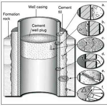
For any CO2 sequestration project, risk is a function of the magnitude of a potential hazard, and the likelihood that the hazard will occur. Leakage is the leading cause of potential hazards. Carbon diox-ide existing as a separate phase may escape from formations, fluids, or carbon capture and transport hardware in many ways (Figure 1-1).

Pipeline failure occurs when a hole is put into the line or there is a rupture in the system; how-ever, the record of CO2 pipelines from 1990 to 2001 shows only 10 accidents without any injuries or fa-talities, which corresponds to a frequency of 3.2x10-4 incidents per km per year (Gale and Davidson, 2003). Unlike natural gas, CO2 is denser than air, so it will not quickly disperse from the point of leakage, therefore creating an increased risk of fatality for individuals in the immediate vicinity of the leak. Since the CO2 is pressurized into liquid form in the pipeline, if there is a rupture, the liquid will freeze before beginning sublimation and moving into the atmosphere. Once injected into a reservoir, the risk of leak-age has the potential to decrease, depending on the efficacy of the Monitoring, Managing and Verifica-tion (MMV) strategies.

Figure 1-1 Possible leakage pathways in an abandoned well

Geologic storage sites are designed to confine all of the injected CO2 over geologic time scales; however, because of the lack of current studies on CO2 leakage and experience with previously engi-neered systems, the IPCC has called for quantitative estimates based on what evidence there is available (Metz, 2005). Pressure and diffusion will primarily drive the subsurface flow of CO2. If the pressure of the CO2 gas is greater than the pore pressure of the caprock, the CO2 will migrate upwards through the caprock (Metz, 2005). Leaked CO2 may reach the water table and migrate into the overlying vadose zone. Here, the pore spaces are filled with water and air, and since CO2 is denser than air, it will displace the air present, leading to potential 100% gas concentrations in the pore volume not filled with water (Oldenburg et al., 2003). The carbon dioxide will continue migrating upwards in this manner until the surface is reached. Similar situations can occur in offshore storage sites, but there the leakage will occur in ocean bottom sediments and then move vertically through the water column.

Carbon dioxide injected into coal seams has the potential to escape through unmapped frac-tures and cleats. CO2 in coal also has the potential to be sorbed into the surrounding strata, and if the pressure system of the coal seam is later reduced, there is potential for the CO2 to desorb from the coal and be released (Pashin, 1991a, Metz, 2005).

et al., 2004). Despite the risk of leakage through abandoned wells, old oil fields may serve as a natural analogue for the ideal sequestration site conditions (Gaus, 2010). This is because they have contained fluids at high pressures effectively for long periods of geologic time.

1.2 Carbon Sequestration

Carbon Capture and Storage (CCS) involves the use of various technologies to collect, concen-trate, transport, and store CO2, with the expressed goal of permanently separating it from the atmos-phere. CO2 can be effectively captured in several different ways. The most typical method involves sep-arating it from a gas stream with techniques like scrubbing the stream with chemical solvents (Siddique, 1990). The reason that gas separation is the most common is because the majority of the research on carbon capture is on the reduction of emissions from a large point source, typically in the energy indus-try.

Another method of carbon sequestration is by ambient capture. Zeman (2007) has proposed a method that involves a scrubber technology that absorbs CO2 directly into a sodium hydroxide solution that is then removed from its alkaline carbonate form into lime, or calcium carbonate. Thermal calcina-tion then removes the CO2 by thermal decomposicalcina-tion (Zeman, 2007). This technology is effective and comparable in energy consumption to gas separation technologies used on coal plants.

1.2.1 Carbon Dioxide

At standard pressure and temperature conditions, CO2 is in a gas state. At low temperatures, CO2 is a solid (a state commonly known as dry ice). At intermediate temperatures (between -56.5˚C and 31.1˚C), CO2 can be liquefied under compression. At temperatures above 31.1˚C, CO2 enters into a su-percritical state where it behaves as a gas with a density approaching or exceeding liquid water. In its dense or liquid phase, CO2 occupies about 0.2% of its original volume of the gas at standard temperature and pressure (STP). This state is ideal for the conveyance of CO2 through pipelines. Figure 1-2 shows the sublimation point, the triple point and the critical point of CO2 (Metz, 2005).

Figure 1-2 CO2 Phase Diagram

Phase diagram modified from (Metz, 2005) showing the critical point where CO2 shifts from gas to liquid and then to a supercritical fluid (striped region) at the critical point which is at 31.1˚C and 1,071 psi.

1.2.2 Carbon Storage

storage in the ocean, and solid state storage (mineralization) by the reaction of CO2 with metal oxides to produce more stable carbonates (Aydin, 2010). Of the options, mineral carbonation has a high cost with great environmental risk. Though injection into deep sea water was one of the earliest proposed meth-ods (Marchetti, 1977), ocean storage is still a poorly understood technology and inherently risky (Aydin, 2010). This leaves carbon capture and geologic storage (CCGS) as the most viable alternative. CCGS has several advantages including (1) a long-standing history of prior research and experience gained from oil and gas exploration which lends itself to immediate applications of CCGS technology (2) large potentials for storage capacity worldwide (3) and having the potential for long-term storage on the scale of thou-sands of years or more.

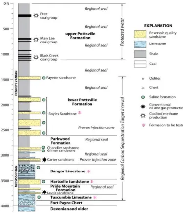
1.3 Purpose of the Study

serve as a regional seal over proven injection zones, making them ideal targets for testing (http://www.netl.doe.gov/publications/proceedings/10/rascp/Alabama_Clark.pdf).

Figure 1-3 Proposed Geologic CO2 Sequestration Interval - Black Warrior River Basin, Alabama

1.4 Previous Research

Marchetti (1977) was one of the first researchers to propose the mitigation of atmospheric CO2 by injecting it into ocean currents with temperatures between 0-10˚C, which would carry the CO2 deep into the ocean for more permanent storage. However, this method is inherently risky. When CO2 in a gas state contacts water, it will dissolve into the water until equilibrium is reached (Drever, 1997). The solubility of CO2 in water, according to Henry’s Law, depends on temperature, the partial pressure of the gas over the liquid, the nature of the water and of the gas (Drever, 1997). The reaction between the dissolved CO2 and the water produces a weak acid, carbonic acid (H2CO3):

CO2 + H2O = H2CO3 Equation 1-1 Carbonic Acid Formation

As the amount of carbonic acid in the water increases, the pH of the water will be driven down, becoming more acidic. Natural waters have a pH of about 5-7, but as the acid is introduced, it increases the pCO2, and the pH can be driven down to 3-4 (Drever, 1997, Deocampo and Ashley, 1999).

These lower pH ranges will have a direct effect on marine ecosystems. No controlled experi-ments in the deep ocean have been performed. However, it is predicted that ecosystem consequences will increase proportionally to the amount of CO2 in the system (Metz, 2005). This can lead to natural buffering caused by the release of calcium carbonate (CaCO3) from the shells of marine organisms. The increase in CO2 composition in the water also can cause an accumulation of CO2 in marine animals, which can lead to death (Metz, 2005).

The mixing of CO2 into reservoir brine has been found to change the brine density and pH over time (Kumar et al., 2008). The same study modeled changes in the water rock interactions and found they occurred rapidly at first but after that, only slower mineral reactions shifted the brine chemistry. This places an emphasis on the need to model the dissolution and precipitation reactions that could sig-nificantly alter rock-fluid properties of the reservoir rocks or the caprocks.

Just like with the dissolution of calcium carbonate bearing marine animals, carbonate and sul-phate minerals, which are characterized by fast reaction times, will quickly dissolve into the CO2 saturat-ed brine and will continue to do so until equilibrium is reachsaturat-ed and could produce secondary reactions like the precipitation of gypsum (Gaus, 2010). The brine, even after pH buffering from carbonate disso-lution, will be strong enough to attack alumino-silicate minerals, which are abundant in sedimentary rocks (Gaus, 2010). Wigand (2008) observed an increased aluminum (Al) and Silica (Si) brine composi-tion in simulated geological sequestracomposi-tion condicomposi-tions, which confirms the dissolucomposi-tion of aluminosilicates. An example of the alteration of clay minerals where CO2 becomes trapped in clay was given by Gaus (2010):

Fe2.5Mg2.5Al2Si3O10(OH)8 + 2.5CaCO3 + 5CO2↔ 2.5FeCO3 + 2.5MgCa(CO3)2 + Al2Si2O5(OH)4 + SiO2 + 2H2O

Chlorite Calcite Siderite Dolomite Kaolinite Chalcedony

CO2 storage. Rapid kinetic reactions, like those of carbonates and some sulphates, can be directly quan-tified in the laboratory, but slower reactions, like those involving aluminosilicates, are not well known at reservoir conditions (Gaus, 2010) and need to be calculated using a variety of models.

The methods relevant to this research are the ones produced in laboratory settings, exhibiting the effects of brine and CO2 on minerals at geological sequestration conditions. To understand the ef-fects of salinity on mineral dissolution, Shao et al. (2011b) ran a series of experiments on phlogopite (KMg3AlSi3O10(OH)2) where brines of various percent composition NaCl were used. It was found that brines of lower salinity more rapidly dissolved phlogopite and in turn formed silica-rich nanoparticles of secondary minerals at higher rates and abundance, and these nanoparticles were predicted to have the capacity to change the physical properties of rocks.

Hu et al. (2011) found in reactions with isolated biotite in supercritical CO2 conditions with brine,

biotite dissolution occurred at increasing rates over a 96 hour period. During this reaction time, accord-ing to XRD and EDS data, secondary precipitation of fibrous illite and kaolinite occurred. This is im-portant because the formation of fibrous illite has been shown to reduce permeability if hydrocarbon reservoirs (Hu et al., 2011) and could severely affect the injection potential of a sequestration site.

Credoz et al., (2011) showed that mixed-layered illite-smectites reacted in the presence of po-tassium feldspar showed that pH had a direct control on the degree of illitization of the mixed-layer mineral. In this study, it was shown that higher pH induced a ‘proton-promoted’ illitization process. When pH was lowered, the illitization of the mixed-layered mineral slowed and the reaction was sug-gested to be more pressure driven.

(Almeu et al., 2011), being that carbonates are more reactive to low pH, high temperature conditions. Common components of shale, illite, smectite, and chlorite, are also shown to dissolve in the laboratory simulations (Almeu et al., 2011, Liu et al., 2012). Mineral precipitations of illite, smectite and carbonates were also common amongst the caprock studies, and were identified by SEM/EDS and XRD.

It is important to emphasize the lack of a common approach. All experiments (e.g., Almeu et al.,

2011, Credoz et al., 2011, Hu et al., 2011, Shao et al., 2011b, Liu et al., 2012) used different pressures,

temperatures, pH ranges, starting brines, and mineral compositions. No common approach to the la-boratory analysis of the effects of geological CO2 sequestration conditions on reservoir rocks or common minerals found in those reservoirs was unveiled in the development of this research. Therefore, though end results might be comparable, the kinetic pathway to that end is not necessarily the same.

1.5 Geological Setting

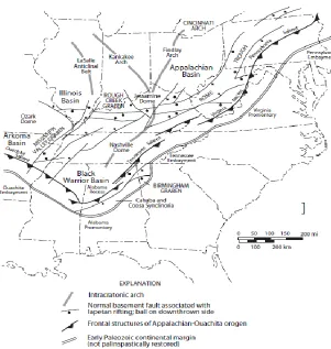
1.5.1 Black Warrior Basin

Figure 1-4 Tectonic setting of the Black Warrior foreland basin. Source: (Thomas, 1988; Pashin and Gastaldo, 2009)

1.5.1.1 Pottsville Formation

The Pottsville Formation is over 3000 meters thick, and is found in the center of the Black War-rior Basin (Hewitt, 1984), and progressively thins to the north as a product of depositional thinning and post-Pennsylvanian erosion (Demko and Gastaldo, 1992). Early Pennsylvanian subsidence of the Appa-lachian thrust belt created space for the Pottsville Formation, which is said to be Westphalian A in age (Demko and Gastaldo, 1992). Westpahalian A fell at the beginning of the Pennsylvanian and lasted for about 10 Mya (315-305 Ma).

The upper Pottsville is a siliciclastic succession containing vertically stacked 4th-order parase-quences (Pashin, 2004, 2007), meaning separase-quences that occur less than every one million years. The up-per portion of the formation is dominated by coal beds and marginal-marine and non-marine sand-stones and shales, while the lower portion is dominated by marine shales (Pashin, 2007).

1.5.1.2 Parkwood Formation

Figure 1-5 Mississippian Stratigraphy of the Black Warrior Basin

Stratigraphic cross section of the Black Warrior basin from northeast Alabama to east-central Mississippi. This section shows the lower Pottsville Formation in contact with the Parkwood Formation. (from Pashin,

1994)

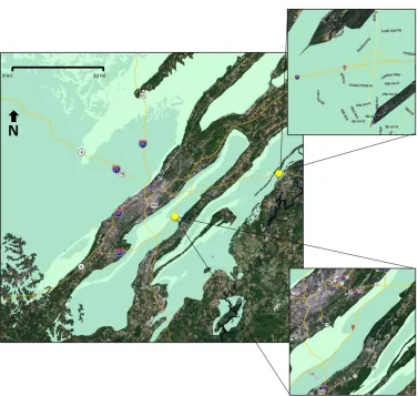
1.5.2 Sample Location

Figure 1-6 Sample Locations

Alabama Geological Survey Map showing sample locations around the Birmingham Area Parkwood Formation (top) (33˚36’42.44” N, 86˚17’ 14.46”W)

Pottsville Formation (bottom) (33˚27’28.92”N, 86˚42’56.78”W)

2 EXPERIMENT

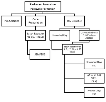
2.1 Procedural Overview

Figure 2-1 Flow diagram of project design.

2.2 Sample Analysis Methods

2.2.1 Thin Section Preparation

Samples of both the Pottsville and Parkwood Formations were prepared by Spectrum Petro-graphics, Inc.

2.2.2 XRD Analysis

X-ray diffraction (XRD) is the instrumentation typically used for the identification of clay miner-als. Diffraction occurs when the wavelength of the X-radiation is roughly the same as the d-spacing of the clay mineral. Bragg’s Law gives the angles for coherent and incoherent scattering from the crystal

Parkwood Formaiton Pottsville Formation

Thin Sections _Preparation Cube

Batch Reaction for 160+ hours

SEM/EDS

Clay Seperation

Unwashed Clay

Batch Reaction for 3, 8, 12, 17, 24, 48,

72 hours

Clay Washed with 0.1M Sodium

Acetate

Batch Reaction for 3, 8, 17, 24, 45, 70

hours

Unwashed Clays XRD

AA for all fluid types. (Si, K)

lattice of a clay mineral. According to Bragg’s Law, when there is constructive interference the diffrac-tion and subsequently the d-spacing of the clay mineral can be calculated using the following equadiffrac-tion:

Equation 2-1 Bragg's Law derived.

Where:

̅̅̅̅

This equation is derived from Figure 2-2:

Where:

S ̅̅̅̅ _̅̅̅̅

̅̅̅̅

̅̅̅̅

̅̅̅̅ ̅̅̅̅

̅̅̅̅ ̅̅̅̅ ̅̅̅̅̅̅̅̅̅̅̅̅̅̅̅̅̅̅̅̅̅̅̅

Z

C

B A

= d = ̅̅̅̅

To generate X-rays, a cathode with a tungsten filament is heated and electrons are emitted across an X-ray tube at -35kV. The tube is held in a vacuum to permit electron acceleration without ion-ization. After crossing the tube, the electrons hit a copper anode and are diffracted, emitting character-istic and continuous radiation. Charactercharacter-istic radiation is emitted when an electron is knocked out of the K-shell and another ‘falls’ in from the second L-shell (L2) (Figure 2-3) (Moore and Reynolds, 1997). This drop in the electron causes the emission of an X-ray photon with characteristic CuK2 radiation. The beam then passes through a beryllium window where radiation such as heat and tertiary X-rays are fil-tered out. The beam then passes through a monochromater, which limits and directs the beam before it hits the sample (Moore and Reynolds, 1997). The beam then penetrates the sample lattice structure and is scattered by the atoms creating constructive and destructive interference. Constructive interfer-ence occurs when two or more rays are in phase and destructive interferinterfer-ence occurs when the rays are out of phase (Moore and Reynolds, 1997). When the atoms are not evenly spaced within the lattice, constructive interference cannot occur and therefore no diffraction takes place (Moore and Reynolds, 1997). The beam is adjusted so that only K is diffracted off of the sample, then through another mono-chromater. At this point, the beam enters a databox for analysis.

X-ray photon emitted from electron drop Displacer Electron

Electron knocked from K-shell

N ucleus K

-shell

L -shell

M -shell Nucleus

K-Shell L-Shell M-Shell

Electron Drop

Figure 2-3 Characteristic Radiation

Two X-Ray diffractometers were used to analyze the samples. The first instrument used was a Philips X-ray Diffractometer with a MDI Databox for computer control and acquisition of diffraction data. The diffractometer was operated at a power rating of 700 Watts and measurements were taken at a step size of 0.02 degrees 2 and a step time of 2 seconds from 5-15 degrees 2 . The software used for data collection was TALK, and for analysis, JADE. The second instrument used was a PANalytical X’pert Pro. The diffractometer took measurement from 2-32 degrees 2 with a 0.007 degree step size and a scan step time of 8.67 seconds. The software used for data collection was the PANalytical software, Da-ta Collector, and for analysis, High Score Plus.

Oriented slides were prepared to promote basal diffraction, or 00l reflections. For phyllosili-cates, this is the most diagnostic method of slide preparation (Moore and Reynolds, 1997). Random mounts were prepared for whole rock analysis following Moore and Reynolds (1997). The X-ray pat-terns were interpreted for clay mineralogy information from Moore and Reynolds (1997). Relative abundances of the minerals found in each sample were quantified using the intensities of the il-lite/smectite (001), illite (001), and kaolinite (002) peaks (Equation 2-2). The values produced from this method are not accurate quantitative estimates, but relative indicators of a change in mineralogy (Spötl

et al., 1993).

Equation 2-2 Relative Abundance Calculation

the peaks. Data collected from the Philips X-ray Diffractometer is not included in the body of the analy-sis, but in Appendix C - Phillips X-Ray Diffractometer Data.

2.2.3 XRF Analysis

Wavelength dispersive (WD) X-ray florescence (XRF), much like XRD, is an analytical technique that introduces a solid sample to an X-ray source (LaTour, 1989, Billets, 2006). The source X-rays have the appropriate energy to cause the sample to emit characteristic X-rays. A qualitative elemental analy-sis is possible from the wavelength of the characteristic radiation, and a quantitative analyanaly-sis is possible by analyzing the intensity of a given wavelength (Billets, 2006). K lines are typically used for elements with atomic numbers from 11 to 46, and L lines are used for elements above atomic number47. M-shell emissions are measurable only for metals with an atomic number greater than 57 (Billets, 2006).

Figure 2-4 WDXRF Spectrometer

(Panalytical, http://www.panalytical.com/index.cfm?pid=313)

The instrument used to perform an XRF analysis was an automated Rigaku 3270 X-ray Spec-trometer fitted with a Rhodium X-ray tube. The instrument was operated at 50 kV and 50 mA. Compan-ion software specifically designed for the Rigaku 3270 X-ray Spectrometer was used for analysis. A ref-erence disk was initially tested to minimize any analytical error, namely the interfref-erence of distinct ele-ments causing the absorption or enhancement of fluorescent radiation or spectral overlap. This refer-ence disk, or ‘alpha correction,’ was used to ensure a linear calibration curve (LaTour, 1989). The Rigaku 3270 system automatically performed calculations to correct for overlap and mass absorption effects, and peak intensities measured by the spectrometer were converted to oxide concentrations by the companion software (LaTour, 1989).

2.2.3.1 XRF Data Treatment

∫

Equation 2-3 Calculation of structural formula From Moore and Reynolds (1997)

2.2.4 AA Analysis

Absorption Spectrometer 3110 was used to analyze all sample solutions. The Perkin Elmer Atomic Ab-sorption Laboratory Benchtop (1985) software program processed the data.

2.2.5 SEM/EDS Analysis

A scanning electron microscope (SEM) functions by bombarding the sample with primary elec-trons in a scanning pattern (Figure 2-6). A beam of elecelec-trons is produced at the top of the microscope by an electron gun. The electron beam follows a vertical path through the microscope, which is held within a vacuum. The striking electron causes the emission of secondary electrons. The height and slope of the object determine the number of secondary electrons generated per unit time, and the ve-locity of those electrons. The beam hitting the sample causes electrons and X-rays to be ejected from the sample. Detectors collect the X-rays, backscattered electrons, and secondary electrons and convert them into a signal that is translated to an image produced on a screen similar to that of a television (Io-wa State University, 2009). This is the final image produced for analysis.

Figure 2-5 Anatomy of a SEM

Figure 2-6 Example of characteristic scattering

From: http://www.purdue.edu/rem/rs/sem.htm#2

All samples were sputter coated with a carbon film, analyzed using a LEO 1450 VP Scanning Elec-tron Microscope (SEM)and were also analyzed using Energy-dispersive X-ray spectroscopy (EDS). Frag-ments of the whole rock were used for SEM/EDS analysis. SEM accelerating voltage was set at 20.0 kV. Probe current for EDS was 5 nA with a beam current 80 mA. Software used to analyze the SEM was Zeiss Smart SEM, EDS analytical software was IXRF 'Iridium'.

2.3 Sample Preparation

2.3.1 Clay Preparation

Whole rock samples were crushed and then powdered in a shatterbox. Samples were disaggre-gated with a Branson Sonifier. Roughly 15 mL of sample were added to 200 mL of diH2O and sonified at 71% amplitude for five minutes. The sample was then centrifuged at 1000 rpm for 5 minutes to remove the sample fraction >1µm. The supernatant was then centrifuged again at 8500 rpm for 20 minutes to separate the fluid from the remaining fine grained sample. This method roughly follows Moore and Reynolds, 1997 and Deocampo et al. 2010.

2.3.1.1 Sodium Acetate Wash

sodium acetate solution and stirred for 0.5 hours. Samples were then filtered through a 0.4 µm Milli-pore filter and then added to 200 mL of diH2O. To reverse the effects of flocculation, samples were soni-cated in the diH2O at 70% amplitude for two minutes. Samples were filtered with a 0.4 µm filter for a second time before they were dried at 90° C for 24 hours, ground with a mortar and pestle and stored in a desiccator. This was done to allow for a comparison of the brine of the untreated clay with the brine of the treated clay, post- experiment.

2.3.2 Cube Preparation

Random samples of both the Pottsville and the Parkwood Formations were cut into one centi-meter cubes for experimentation. The cubes were then treated in the batch reactor with just brine or brine and supercritical CO2. Reaction times were between 159-167 hours. This method came from Massarotto et al. (2010), but the remainder of the laboratory procedure was not followed. Massarotto

et al. (2010) observed the changes in permeability and crystalinity in coal that came with exposure to

diH2O and CO2.

2.3.3 Batch Reactions

A Parr Instruments High Strength Acid Digestion Vessel was used to run the experiment in a Lindberg/Blue electric oven. The digestion vessel contained a 23 mL Teflon cup. Teflon cups were pre-treated with so as to test the amount of absorption into the porous cup (Giammar et al., 2005). The pre-treated cup was weighed before the application of and after. No significant change in weight occurred (Table 2-1), so the treatment was not used again.

Table 2-1 Treatment of Teflon Cups with CO2

Pre-Treatment Weight Mass Post-Treatment

Suspended concentrations of clay were held between 20g/L and 30g/L (following Gimmar et al, 2005), meaning that 0.4-0.5g of sample were added. Variation in sample mass was considered insignifi-cant. Given that the average density of silicates is about 2.65 g/cm3, the mass of sample added would result in a change of volume between 0.15-0.20 mL using the following formula:

Equation 2-4 Formula to calculate the total volume of clay.

This change in volume was considered to be small enough that small changes in the mass of the sample would not have significantly altered the pressure inside of the vessel.

Weighed portions of were used to produce 120+ bar pressure within the Teflon cup at 90°C. Pressure calculations are shown in Appendix B - Batch Reaction Pressure Calculations. The volume of the container was 23 mL and 5 mL was left for headspace . In order to maintain the standard con-centrations, 0.5 g of solids was added to 18 mL of brine. The brine was first frozen in the cup so as to prevent the rapid sublimation of the dry ice.

Equation 2-5 Ideal Gas Equation

Where:

Clay samples were subjected to the simulated sequestration conditions over 3, 8, 17, 24, 45, and 70 hour time periods, and whole rock cubed samples were subjected for 165+ hours (Appendix F). The time required for the temperature of the digestion vessel to reach 363K was not taken into account. Parr Instruments High Strength Acid Digestion Vessel is a closed system which prevented the measure-ment of the temperature inside of the Teflon cup during experimeasure-mentation; therefore, the exact time of temperature equilibration was not known. After the experimental run time, the vessel was allowed to cool for an hour in order to reduce the pressure and temperature of the instrument so that it could be opened. The samples were then filtered and prepared accordingly.

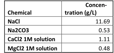
2.3.4 Brine Composition

Table 2-2 Brine Composition

Chemical

Concen-tration (g/L)

NaCl 11.69

Na2CO3 0.53

CaCl2 1M solution 1.11

MgCl2 1M solution 0.48

2.3.5 XRD Sample Preparation

Samples not rinsed by sodium acetate were used for the XRD experiments. After the reaction, samples were wet mounted on slides and analyzed using XRD.

2.3.6 XRF Sample Preparation

The sample preparation roughly followed the methodology outlined by La Tour (1989). Prior to XRF disc preparation, a loss on ignition was performed at 1100˚C for 60 minutes. This was done to re-move any excess organic matter or water from the clay structure. Fused discs were prepared for analy-sis because fused discs allow a homogenous distribution of elements. This ensures a more accurate analysis of the sample. To make the fused disk, 0.5 g of sample was added to 4.5 g of lithium tetra-borate. This mixture was heated in a 95% Platinum (Pt), 5% Gold (Au) crucible at 1000˚C for 15 minutes in a high temperature furnace, including a stirring period at 10 minutes. This homogenous mixture was then poured into a preheated mold to form the sample disc. Once the disc was formed, it was stored in a desiccator.

2.3.7 AA Sample Preparation

Thus a finer filter was required (0.2 µm) for filtrations handling the sodium acetate washed clay. During the AA testing of the brines, it was noticed that ions, specifically K, were sticking to the sides of the test tubes, and skewing the results. Therefore, one drop of laboratory grade nitric acid was added to each sample tube to prevent cation adsorption to the surface of the bottles.

2.3.8 SEM/EDS Sample Preparation

Cubes of both the Pottsville and Parkwood post-experimental procedure were broken into small fragments for analysis. Samples were treated with a thin carbon film prior to analysis and mounted so that the interior portion of the cube would be analyzed.

3 RESULTS

3.1 Thin Section

3.1.1 Pottsville Formation

Figure 3-1 Pottsville Formation in Cross Polarized Light (100x)

Figure 3-2 Pottsville Formation Sedimentary Structures (actual size)

A.) Flame Structure (B.) Ball and Pillow Structure (C.) Cross-bedding

A

B

3.1.2 Parkwood Formation

In thin section, the Parkwood Formation shows very large quartz crystals caught in a fine-grained matrix (Figure 3-3). The sedimentary structures of the Parkwood formation are more simple than the Pottsville Formation, with only cross-bedding present (Figure 3-4).

Figure 3-3 Parkwood Formation in Cross-polarized Light (100x)

Figure 3-4 Parkwood Formation Sedimentary Structures (2x)

A.) Cross-bedding

3.2 Whole Rock Mineralogy

Random mounts of both the Pottsville and the Parkwood formations were graphed using High Score, and clay mineral estimations were made using the software as well. The Pottsville Formation was shown to have a mixture of muscovite, vermiculite, and quartz. The Parkwood Formation was shown to have the same composition. Individual peaks are labeled and identified in Appendix D - PANalytical X-Ray Diffraction . These identifications however are incorrect. The identification of muscovite is actually the recognition of a 10 Å clay, illite. The identification of vermiculite is actually the recognition of the 14 Å phase of a clay, chlorite.

Figure 3-5 Pottsville Whole Rock XRD Pattern

0 2000 4000 6000 8000 10000 12000 14000

5 15 25 35 45 55 65

In

te

n

si

ty

2

Figure 3-6 Parkwood Whole Rock XRD Pattern

3.3 Fluid Chemistry

Ions of potassium (K) and silica (Si), previously absent in the starting brine solution, appeared in all solutions at 3, 8, 17, 24, 45, and 70 hours, indicating the dissolution of reacting solids (raw data avail-able in Appendix G - Atomic Absorbance Data). Rapid dissolution of both silica and potassium were evident in each sample. The amount of each cation entering solution is given in Table 3-1.

Silica, in all cases, quickly entered into the brine, and in less than 20 hours, its dissolution slowed (Figure 3-7). Samples washed with sodium acetate exhibited a slightly higher rate of dissolution, but were proportionally similar to the untreated samples, indicating the same reactions.

0 5000 10000 15000 20000 25000

5 15 25 35 45 55 65

In

te

n

si

ty

2

Figure 3-7 AA Detection of Silica in Brine

Potassium, in all cases, rapidly entered the brine (Figure 3-8). After the first three hours, the amount of potassium showed significantly lower rates of change. The clays washed with sodium acetate exhibited a lower rate of dissolution.

Figure 3-8 AA Detection of Potassium in Brine

0 5 10 15 20 25 30 35 40 45

0 20 40 60 80

m

g/

L

Time

Sillica In Brine

Potsville Washed Pottsville Unwashed Parkwood Washed Parkwood Unwashed 0 5 10 15 20 25 30 35

0 20 40 60

m

g/

L

Time (hrs.)

AA Data - Potassium

Pottsville

Pottsville_Washed

Parkwood

Si and K data suggest that the brine reaches a near equilibrium state around 24 hours after the experimental start time. A comparison of the molar ratio of K:Si in idealized illite (~0.2) to the same ra-tio in the stabilized brine average (

Table 3-1) shows that though illite might be the contributor of K to the brine system, the amount of Si is low and suggests a reprecipitation of a siliceous mineral.

Table 3-1 Si, K Composition of Brine

Exposure Time ppm Si mmol/L Si ppm K mmol/L K Stabilized Average

K/Si

Pottsville Unwashed 0 1.46 0.05 0.29 0.01 1.23

3 9.19 0.33 21.21 0.54

8 13.58 0.48 20.29 0.52

17 17.27 0.61 23.66 0.61

24 17.36 0.62 21.34 0.55

45 14.09 0.50 32.65 0.83 70 16.15 0.58 27.34 0.70

Pottsville Washed 0 1.46 0.05 0.29 0.01 0.39

3 4.73 0.17 8.54 0.22 8 23.11 0.82 11.36 0.29 17 16.93 0.60 10.19 0.26 24 19.33 0.69 10.34 0.26

45 21.31 0.76 10.81 0.28 70 16.84 0.60 10.45 0.27

Parkwood Unwashed 0 1.46 0.05 0.29 0.01 0.69

3 10.05 0.36 28.73 0.73 8 12.80 0.46 28.34 0.72 17 27.32 0.97 25.41 0.65 24 31.19 1.11 29.15 0.75

45 30.24 1.08 30.50 0.78 70 29.47 1.05 27.63 0.71

Parkwood Washed 0 1.46 0.05 0.29 0.01 0.24

3 9.11 0.32 11.39 0.29 8 17.27 0.61 9.95 0.25 17 30.85 1.10 12.01 0.31 24 38.41 1.37 13.55 0.35

45 38.49 1.37 11.75 0.30

70 38.23 1.36 12.98 0.33

3.4 Solid Phase Reactions

3.4.1 XRD Clay Analysis

(001) and illite (001) respectively. The peak around 12.4 2 could represent kaolinite (001) or chlorite (002) or a mixture of both. However, the large peak around 12.4 2 , 7.1 Å likely represents Fe-chlorite (Chamosite) since Fe-chlorite, as opposed to Mg-chlorite, has even peaks which dominate in intensity over the odd peaks (Moore and Reynolds, 1997). The peak located at 18.8 2 4.74 also suggests the presence of chlorite over kaolinite (Moore and Reynolds, 1997). Illite presence is confirmed by its (001) and (002) peaks at 8.8 2 , 10.1 and 17.7 2 , 5.0 . The quartz (022) peak was barely present above the ‘noise’ of the graph, but was accounted for, showing only a faint peak on average around 19.5 2 , 4.2 Å (Moore and Reynolds, 1997).

Figure 3-9 Pottsville Clay Peak Comparison with average d-spacing Angstroms

3 8 13 18 23 28

2 Theta

Pottsville Clay Peak Comparison

Pot_Clay_Average_glycol Pot_3_glycol Pot_8_glycol Pot_17_glycol Pot_24_glycol Pot_45_glycol Pot_70_glycol Fe-C (002) 7.2 I (002)

Figure 3-10 Parkwood Clay XRD Peak Comparison with Average d-spacing in Angstroms

3.4.1.1 Relative Abundance of Clay Minerals

Relative to the illite (001) peak and the kaolinite (002) peak, Fe-chlorite (002) abundance increased in both samples for the first 17 hours before it began to reduce (Figure 3-11). Illite decreased, relatively, before increasing in both samples over the last experimental run time from 45 to 70 hours (Figure 3-12). Kaolinite increased in relative abundance before decreasing during the last experimental run time (Figure 3-13). Although some variations are observed, no wholesale clays are noted, and the basic clay assemblage remains.

2 7 12 17 22 27 32

2 Theta

Parkwood Clay Peak Comparison

PW_Clay_Average_glycol PW_3_glycol PW_8_glycol PW_17_glycol PW_24_glycol PW_45_glycol PW_70_glycol Fe-C (002)

Figure 3-11 Relative Abundance – Fe-Chlorite (001)

Figure 3-12 Relative Abundance - Illite (001)

0 0.05 0.1 0.15 0.2 0.25 0.3 0.35

0 20 40 60 80

R e lativ e A b u n d an ce Time

Fe Chlorite (001)

/(Fe-Chlorite (001)+Ill (001)+Kaol(002)

)

Pottsville Parkwood 0 0.1 0.2 0.3 0.4 0.5 0.6 0.7

0 20 40 60 80

R e lativ e A b u n d an ce Time

Illite (001)

/(Smectite (001)+Ill (001)+Kaol(002)

)

Pottsville

Figure 3-13 Relative Abundance - Kaolinite (002)

3.4.2 XRF data

Octahedral compositions of the clay minerals are shown through the calculation of structural formulas of layer silicates assuming a 2:1 structure formula unit of 11 oxygen atoms (Moore and Reyn-olds, 1997, Deocampo, 2004) (Table 3-2). The Pottsville and the Parkwood formations plot closely on a triplot of their octahedral components (Al, Fe, Mg) (Figure 3-14), but magnesium has very little effect on the octahedral composition of the clay, lending the octahedral sheet to be classified as gibbsite-like. The Octahedral Cation Index (OCI), an expression of the octahedral composition of any clay (Deocapmo, 2004), was plotted against time to demonstrate the lack of change with respect to time (Figure 3-15). One outlier was excluded (Pottsville 3 hr.). Figure 3-16 shows the relation of only Fe and Al with the out-lier, Pottsville 3 hr, excluded. The Pottsville Formation shows a higher ratio of Fe to Al, but there is no significant change in the relation of octahedral composition of these clays to time (Figure 3-17) when excluding Mg from the analysis.

0 0.1 0.2 0.3 0.4 0.5 0.6

0 20 40 60 80

R

e

lativ

e

A

b

u

n

d

an

ce

Time

Kaol (002)

/(Fe-Chlorite (001)+Ill (001)+Kaol(002)

)

Pottsville

Table 3-2 Clay Mineral Structural Compositions

Showing the number of cations per formula unit based on an average structure.

Tetrahedral Octahedral Interlayer Cation OCI

Si Al Al Ti Fe Mg Ca Na K

Pottsville

0 3.27 0.73 1.46 0.05 0.51 0.25 0.02 0.07 0.50 0.13 3 3.31 0.69 4.07 3.35 2.53 2.47 3.89 0.72 1.69 0.37 8 3.23 0.77 1.40 0.06 0.54 0.25 0.04 0.14 0.53 0.13

17 3.28 0.72 1.41 0.05 0.52 0.24 0.08 0.13 0.48 0.13

24 3.27 0.73 1.41 0.05 0.53 0.24 0.08 0.13 0.49 0.13

45 3.27 0.73 1.42 0.05 0.52 0.24 0.07 0.14 0.48 0.12

72 3.27 0.73 1.41 0.05 0.52 0.24 0.09 0.13 0.48 0.12

Parkwood .

0 3.96 0.04 1.42 0.05 0.40 0.18 0.01 0.10 0.29 0.10 3 3.83 0.17 1.39 0.05 0.44 0.20 0.05 0.14 0.31 0.11 8 4.13 0.00 1.27 0.04 0.35 0.16 0.04 0.15 0.25 0.10

17 3.81 0.19 1.37 0.05 0.45 0.20 0.05 0.16 0.32 0.11

24 3.83 0.17 1.41 0.05 0.44 0.19 0.03 0.14 0.31 0.10

45 4.04 0.00 1.36 0.05 0.37 0.17 0.05 0.15 0.26 0.10

72 3.80 0.20 1.37 0.05 0.45 0.21 0.06 0.14 0.32 0.12

Figure 3-14 Tri-Plot of All Experimental Clay Composition

Octahedral Composition of All Experimental Clays

Al

Figure 3-15 Octahedral cation index of clay in relation to time.

Figure 3-16 Octahedral Composition Fe/Al

0.08 0.09 0.10 0.11 0.12 0.13 0.14

0 20 40 60 80

Oct ah e d ral ( M g/ (Al +Fe) ) Time

OCI

0.000 0.200 0.400 0.600 0.800 1.000

Al

Fe

Fe vs. Al Octahedral Composition

Pottsville

Figure 3-17 Fe2O3/Al2O3 vs. Time

Tetrahedral composition of the clays are compared by plotting the number of cations per formu-la unit of Si and Al (Figure 3-18). The individual cformu-lays cluster with a higher ratio of Si to Al in the Potts-ville Formation. There is a greater amount of change in the tetrahedral sheet cations than in the octa-hedral, but nothing significant (Figure 3-19).

Figure 3-18 Tetrahedral Composition

0.000 0.100 0.200 0.300 0.400 0.500 0.600 0.700

0.00 20.00 40.00 60.00 80.00

Fe/

A

l

Time

Fe/Al vs. Time

Pottsville Parkwood 0.0 0.1 0.2 0.3 0.4 0.5 0.6 0.7 0.8 0.9

3.0 3.2 3.4 3.6 3.8 4.0 4.2

Figure 3-19 Tetrahedral Composition vs. Time

3.4.3 SEM/EDS

SEM images coupled with EDS data have produced a qualitative way of looking at sample change. Pottsville Formation (Figure 3-2020 - Figure 3-222) shows a reduction in aluminosilicates and the appearance of dissolution pits, which are included in the sample exposed to the brine without CO2 (Figure 3-211 - Figure 3-222).

The Parkwood Formation shows the loss of an Fe-aluminosilicate, possibly Fe-chlorite, through the EDS data in Figure 3-23-Figure 3-25. The Parkwood Formation also shows a loss of Al, K, and Fe with possible precipitation of amorphous silica. Dissolution pits are also present in the Parkwood formation.

0 0.05 0.1 0.15 0.2 0.25

0.00 20.00 40.00 60.00 80.00

A

l/

Si

Time

Tetrahedral Sheet Change vs. Time

Pottsville

Figure 3-20 SEM image Pottsville Unaltered and EDS

Figure 3-21 Pottsville No CO2 and EDS

Figure 3-22 SEM Image Pottsville CO2 and EDS

Figure 3-23 SEM Image Parkwood Unaltered and EDS

Figure 3-24 SEM Image Parkwood No CO2 and EDS

Figure 3-25 SEM Image Parkwood CO2 and EDS

4 DISCUSSION

4.1 Mineralogy

The High Score output of the random mount whole rock samples differs from interpretations of clay content from Moore and Reynolds (1997). The identification of ‘muscovite’ is most likely the identi-fication of the 10Å clay illite. This misidentiidenti-fication is most likely a function of the sample being a 2- or 3-layer polytype of illite with (001) oriented parallel to the cleavage direction where the dissolution of illite aided in its re-precipitation into the (001) orientation and a slight shift towards the end-member, muscovite (Grub et al., 1991). This would occur as the amount of K and Al increased in the sample. Therefore, it is suggested that High Score’s classification of ‘muscovite’ in both the Pottsville and the Parkwood formations is a function of detrital illite composition moving toward its muscovite

end-member, and should instead be interpreted as illite. Illite identification is confirmed by XRD clay analysis data.

The identification of ‘vermiculite’ is also likely incorrect, and is most likely the identification of the 14Å clay chlorite. Analysis was not performed to confirm or deny the validity of the composition of chlorite. However, this interpretation follows the oriented clay mineral interpretation (Moore and Reynolds, 1997). Additional testing, including saturating the sample with formamide to insure the cor-rect identification of chlorite and not kaolinite or halloysite needs to be done (Moore and Reynolds, 1997).

4.2 Fluid Chemistry

molar ratio K:Si of the brine near equilibrium compared to the same molar ratio of the idealized illite formula suggests; however, that illite is first precipitated into the brine, but then, due to the remaining higher concentrations of K in the brine, silica precipitates out, possibly as amorphous silica as suggested by SEM/EDS data.

Minor fluctuations in brine composition could be attributed to minor differences in sample composition stemming from a non-homogeneous mixture of sample creating varying proportions of clay types in each experimental run. Unfortunately, unless known portions of isolated clays were mixed, there would be no way to prevent this from occurring within the parameters of this experimental meth-od. Having an unknown mixture of clay minerals has created, to a degree, ambiguity in the fluid chemis-try results.

4.3 Solid Phase Reactions

X-ray diffraction data show both the Pottsville and the Parkwood formations are mostly com-posed Fe-chlorite, illite, kaolinite, and quartz. With increasing exposure to CO2 and brine, there is a change in the composition of the clays from both samples that roughly mimic each other, indicating that the change in the clay is not a function of a lack of homogeneity in samples, but instead, a trend in the alteration of clay composition.

In both samples, a decrease in the amount of illite in relation to the amount of Fe-chlorite is in-dicative of the dissolution of illite. Towards the end of the reaction time, the relative abundance of illite increases again, suggesting the reprecipitation of illite. Illite precipitation has been confirmed in the works of Almeu et al. (2011), Credoz et al. (2011), Hu et al. (2011), Shao et al. (2011), and Garcia et al.

(2012).

SEM/EDS data also qualitatively confirms the dissolution of mineral surfaces. The Pottsville and the Parkwood Formations show dissolution pits on mineral surfaces. These surfaces are identified as Fe-chlorite because of the Fe content from the EDS data and its correlation to XRD data. This indicates that smectite was dissolving into solution. Silica abundance increases, indicating the precipitation of amor-phous silica. Though silica typically dissolves at higher pH and the supercritical CO2-brine solution is acidic, the clay-brine interface has a higher pH which leads to the dissolution of silica (Thomson, 1959). Therefore it is hypothesized that the silica is then transported to regions of lower pH, where it is depos-ited.

These results illustrate the need for further study. If dissolution reactions are occurring in geo-logical CO2 sequestration conditions, this will directly affect the permeability of the reservoir and the reservoir seal. Precipitation reactions could restrict the injectivity of a formation by decreasing pore throat diameters. Therefore, it is essential to fully understand the geochemical effects of the brine-rock-CO2 system with respect to time so as to make long-term predictions about the viability of a formation.

5 Future Work

To improve upon the research done in this study, more extensive XRD analytical techniques need to be applied. To verify the presence of chlorite, samples should be heated to 550˚C for one hour to cause dehydroxylation of the hydroxide sheet and shift the (001) reflection from about 6.3 to 6.4 2 and reduce the (002-004) reflections. Air dried sample diffractograms also need to be compared to compare to all forms of treatment. To verify whether the samples contain vermiculite or chlorite with Fe substitution, a treatment of k-saturation is necessary.

qualitative analysis to a quantitative analysis. Using the same sample will show what happens to indi-vidual crystals and the matrix with time and exposure to CO2.

To better understand what actually happens to clay minerals, individual clays must be modeled in water, brine, and brine plus CO2. This will allow for accurate assessments about what is occurring to each clay and help to make accurate predictions about what is occurring to the whole rock in geologic CO2 sequestration conditions.

A full suite of AA or inductively coupled plasma mass spectrometry (ICP-MS) data needs to be collected to quickly and accurately assess what elements are moving into and out of the clay system. This must be performed on samples that have been reacted with water, brine, and brine plus CO2 to show how brine chemistry is affected by the brine composition as well as the addition of CO2 in conjunc-tion with the clay under observaconjunc-tion. The data produced would inform the researcher about when the rock-brine-CO2 system stabilized. In conjunction with other data, like XRF, predictions about the clay fraction of a whole rock can be made.

6 CONCLUSIONS

 This experiment has shown that the clay fractions of caprocks are affected by supercritical CO2

introduction to the simulated pore fluids.

 The major clays identified using XRD are Fe-chlorite, illite, smectite and kaolinite.

 Reactions of the mixture of clay-brine-CO2 are documented by changes in the aqueous

chemis-try relative to the starting brine.

 The brine composition stabilized within 70 hours, indicating the clay-brine-CO2 system will

equil-ibrate at some point, which is determined by the composition of the clay-brine system.  Dissolution of the clay minerals was illustrated by XRD and SEM/EDS results.

 SEM/EDS results also suggest the precipitation of silicate minerals.

 XRF data suggests congruent dissolution precipitation reactions as the main catalyst for change

in the clay system since there is no major change recorded in the structural formula of the tet-rahedral or octahedral structure of either clay.

 While each method of observing the changes in clay mineralogy indicated some change, or lack

thereof, the observations between methods were not totally parallel because each method ob-serves the sample on a different scale.

 The current data calls for further research into the long-term stability of all potential formations

REFERENCES

Allinson, W. G., Nguyen, D.N., Bradshaw, J., 2003, The Economics of Geological Storage of CO2 in Australia: APPEA Journal, p. 623.

Almeu, B. L., Aagaard, P., Munz, I.A., Skurtveit, E., 2011, Caprock interaction with CO2: A laboratory study of reactivity of shale with supercritical CO2 and brine: Applied Geochemistry, v. 26, p. 1975-1989.

Aydin, G., Karakurt, K, Aydiner, K., 2010, Evaluation of geologic storage options of CO2: Applicability, cost, storage capacity and safety: Energy Policy, v. 38, p. 5072-5080.

Billets, S., 2006, XRF Technologies for Measuring Trace Elements in Soil and Sediment: EPA Innovative Technology Verification Report.

Bock, B., Rhudy, R, Herzog, H., Klett, M., Davidson, J., Della Torre Ugarte, D., Simbec, D., 2003, Economic Evaluation of CO2 Storage and Sink Options: DOE Research Report.

Chadwick, R. A., Zweigel,T. Gregersen, U., Kirby, G.A. Holloway, S., Johannessen, P.N., 2004, Geological reservoir characterization of a CO2 storage site: The Utsira Sand, Sleipner, northern North Sea: Energy, v. 29, p. 1371-1381.

Credoz, A., Vildstein, O., Jullien, M., Raynal, J., Trotignon, L., Pokrovsky,O., 2011, Mixed layer illite smectitie reactivity in acidified solutions: implications for clayey caprock stability in CO2 geological storage: Applied Clay Science, v. 53, p. 402-408.

Demko, T. M., Gastaldo, R.A., 1992, Paludal environments of the Mary Lee coal zone, Pottsville Formation, Alabama: stacked clastic swamps and peat mires: International Journal of Coal Geology, v. 20, p. 23-47.