Simulation and validation of concentrated subsurface lateral flow paths in an agricultural landscape

© Author(s) 2009. This work is distributed under the Creative Commons Attribution 3.0 License.

Earth System

Sciences

Simulation and validation of concentrated subsurface lateral flow

paths in an agricultural landscape

Q. Zhu and H. S. Lin

The Pennsylvania State University, Department of Crop and Soil Sciences, 116 Agricultural Sciences and Industry Building, University Park, PA 16802, USA

Received: 28 February 2009 – Published in Hydrol. Earth Syst. Sci. Discuss.: 1 April 2009 Revised: 5 August 2009 – Accepted: 7 August 2009 – Published: 20 August 2009

Abstract. The importance of soil water flow paths to the transport of nutrients and contaminants has long been recog-nized. However, effective means of detecting concentrated subsurface flow paths in a large landscape are still lack-ing. The flow direction and accumulation algorithm based on single-direction flow algorithm (D8) in GIS hydrologic modeling is a cost-effective way to simulate potential con-centrated flow paths over a large area once relevant data are collected. This study tested the D8 algorithm for simulating concentrated lateral flow paths at three interfaces in soil pro-files in a 19.5-ha agricultural landscape in central Pennsyl-vania, USA. These interfaces were (1) the interface between surface plowed layers of Ap1 and Ap2 horizons, (2) the in-terface with subsoil water-restricting clay layer where clay content increased to over 40%, and (3) the soil-bedrock in-terface. The simulated flow paths were validated through soil hydrologic monitoring, geophysical surveys, and observable soil morphological features. The results confirmed that con-centrated subsurface lateral flow occurred at the interfaces with the clay layer and the underlying bedrock. At these two interfaces, the soils on the simulated flow paths were closer to saturation and showed more temporally unstable moisture dynamics than those off the simulated flow paths. Appar-ent electrical conductivity in the soil on the simulated flow paths was elevated and temporally unstable as compared to those outside the simulated paths. The soil cores collected from the simulated flow paths showed significantly higher Mn content at these interfaces than those away from the sim-ulated paths. These results suggest that (1) the D8 algorithm is useful in simulating possible concentrated subsurface

lat-Correspondence to: H. S. Lin

([email protected])

eral flow paths if used with appropriate threshold value of contributing area and sufficiently detailed digital elevation model (DEM); (2) repeated electromagnetic surveys can re-flect the temporal change of soil water storage and thus is a useful indicator of possible subsurface flow path over a large area; and (3) observable Mn distribution in soil pro-files can be used as a simple indicator of water flow paths in soils and over the landscape; however, it does require suffi-cient soil sampling (by excavation or augering) to possibly infer landscape-scale subsurface flow paths. In areas where subsurface interface topography varies similarly with surface topography, surface DEM can be used to simulate potential subsurface lateral flow path reasonably so the cost associated with obtaining depth to subsurface water-restricting layer can be minimized.

1 Introduction

Contribution of concentrated subsurface lateral flow in soils to rapid transport of nutrients and chemicals has been well recognized (e.g., Tsukamoto and Ohta, 1988; Elliot et al., 1998). Therefore, generating three-dimensional (3-D) scheme of subsurface flow paths in a landscape can help nutrient management and pollution control. However, lim-ited means are available for detecting (especially nondestruc-tively) subsurface flow paths in a large landscape. In addi-tion, most studies on concentrated subsurface lateral flow re-ported in the literature have been conducted in forested catch-ments (e.g., Kitahara et al., 1994; Sidle et al., 2001; Lin et al., 2006), with much fewer studies conducted in agricultural landscapes.

The soil-bedrock interface has been recognized in a num-ber of recent studies as an important concentrated subsurface

lateral flow path. For example, Freer et al. (1997) reported a positive correlation between total flow volume and the contributing area calculated from a digital elevation model (DEM) of the soil-bedrock interface (instead of the soil sur-face). Noguchi et al. (1999) demonstrated through dye trac-ing that bedrock topography was important in contributtrac-ing to preferential flow in a forested hillslope. Buttle and McDon-ald (2002) found that water flow at bedrock surface occurred in a thin saturated layer. Haga et al. (2005) demonstrated that saturated subsurface flow above the soil-bedrock inter-face was dominant subsurinter-face runoff. Fiori et al. (2007) also reported that the principal mechanism for the stream flow generation was subsurface flow along the soil-bedrock inter-face.

Significant changes in texture, structure, and bulk density can often be observed across the boundary of two adjacent soil horizons in a soil profile. Therefore, soil horizon inter-face can alter water flow direction and pattern (e.g., Kung, 1990, 1993; Ju and Kung, 1993; Gish et al., 2005; Lin et al., 2006). Several studies have reported water accumulation and subsequent lateral preferential flow above a high clay con-tent and low hydraulic conductivity B horizon (called argillic horizon) (e.g., Haria et al., 1994; Perillo et al., 1999; Heppell et al., 2000). Slowly-permeable fragipans in many soils have been recognized to develop seasonal perched water table and thus trigger lateral preferential flow (e.g., Palkovics and Pe-terson, 1977; McDaniel et al., 2008). Because of compaction caused by farming equipments, plowpan (Ap2 horizon) un-derneath plowed layer (Ap1 horizon) can potentially gener-ate lgener-ateral seepage, especially in rice paddy soils (e.g., Chen et al., 2002; Sander and Gerke, 2007). Sidle et al. (2001) also observed lateral flow at organic horizon–mineral soil in-terface in forested hillslopes.

Although concentrated subsurface lateral flow at the inter-faces between soil horizons and between soil and underly-ing bedrock are important to water flow and chemical trans-port across a landscape, methods for effectively determining where and when concentrated subsurface lateral flow occurs remain very limited. In recent years, flow direction and accu-mulation siaccu-mulations based on DEM have been implemented in Geographic Information System (GIS) hydrologic mod-eling tools (e.g., Maidment, 2002). These simulations are based on single-direction flow algorithm (D8) (also called steepest gradient algorithm) (O’Callaghan and Mark, 1984). The D8 algorithm has been widely used in the simulation of surface flow paths (e.g., Marks et al., 1984; Jones, 2002; Sch¨auble et al., 2008). However, it has not been widely used to simulate subsurface flow paths at different interfaces, al-though some studies have used other algorithms (e.g., MD8 and Dinf) to predict groundwater level thus groundwater flow (e.g., Zinko et al., 2005; Sørenson et al., 2006). Gish et al. (2005) have used the D8 modeling tool to identify con-centrated subsurface lateral flow paths above the clay layer in an agricultural watershed, which were confirmed by ground penetration radar (GPR) investigations. Bakhsh and Kanwar

(2008) reported that flow accumulation generated from the D8 method contributed significantly to discriminate subsur-face drainage clusters.

However, the D8 method only allows one of eight flow directions, which constrains the representation of flow path variability (Fairfield and Leymarie, 1991). Flow path simu-lated using the D8 tends to be concentrated to distinct, often artificially straight lines, as reported by Seibert and McGlynn (2007). In addition, Kenny et al. (2008) pointed out that the D8 algorithm can not yield good simulation results in low relief areas or areas with poor DEMs. Efforts to alleviate these drawbacks have focused on introducing models with multiple-flow directions, also called dispersive algorithms. For example, the algorithm proposed by Quinn et al. (1991) (MD8) distributes flow to all neighboring downslope cells weighted according to slope. However, dispersive algorithms produce numerical dispersion from a DEM cell to all neigh-boring cells with a lower elevation, which may be inconsis-tent with the physical definition of upstream drainage area (Orlandini et al., 2003). Tarboton (1997) proposed a nondis-persive algorithm (Dinf) that assigns flow direction angle be-tween 0 and 2πradian and allows an infinite number of pos-sible flow directions. However, a certain degree of dispersion still remains in this method (Orlandini et al., 2003). Seibert and McGlynn (2007) incorporated and extened the MD8 and Dinf models and generated a new triangular multiple flow di-rection algorithm (MD∞) that takes the advantages of both models. According to Paik (2008), dispersive algorithms cannot define specific flow paths (nondispersive); therefore they are not suitable for investigating the transport of nutri-ent, pollutant, and water through channel corridors. In this respect, nondispersive algorithms (e.g., D8) are preferable. However, other studies also showed that the dispersive al-gorithms can be used to define dispersive flow paths (e.g., Bogaart and Troch, 2006). A few studies have suggested that the D8 method can yield good results in areas of substantial relief using a high resolution DEM (e.g., 3–5 m resolution DEM) (Guo et al., 2004; Kenny et al., 2008; Paik, 2008; Wu et al., 2008).

of soil ECa measured repeatedly within a short period of time (e.g., within a few months) should reflect the temporal vari-ation in soil water content, after temperature correction (Zhu et al., 2009).

Soil morphological features (e.g., redox features, soil structure, macropores, and many others) are indicative of soil water movement (Lin et al., 2005). For example, pre-vious studies have suggested that soil manganese (Mn) con-tent is a good indicator of water movement in soil profiles. This is because Mn can be easily reduced and mobilized with moving water, and then oxidized and re-deposited when soil dries and O2reenters the soil (Patrick and Henderson, 1981).

Yaalon et al. (1977) found that soil Mn content was topog-raphy and drainage related in three catenas. McDaniel and Buol (1991) and Walker and Lin (2008) reported greater soil Mn content at footslope and concave landscape positions be-cause of water accumulation. Cassel et al. (2002) reported a positive relationship between subsurface flow paths and dis-solved Mn along hillslopes. However, such simply indicator has not been utilized in larger scale studies (e.g., catchment and farm scales) to interpret landscape–scale subsurface wa-ter movement.

The objective of this study was to investigate the reliabil-ity of high-resolution DEM-derived flow direction and accu-mulation algorithm (D8) implemented in ArcGIS 9.2 (ESRI, Redlands, CA, USA) for simulating concentrated subsurface lateral flow paths at three interfaces in a large agricultural landscape. The interfaces investigated included (1) the in-terface between the surface layers of Ap1 and Ap2 horizons, (2) the interface between the upper soil profile and subsoil clay layer where clay content increased to over 40%, and (3) the interface between soil and the underlying bedrock. Three field indicators were then used to validate the simulated flow paths, including field soil moisture monitoring, EMI surveys, and soil Mn content observation at these interfaces.

2 Materials and methods

2.1 Study site

This study was conducted in an agricultural landscape typ-ical of the valley in the Northern Appalachian Ridges and Valleys Physiographic Region in the USA (Fig. 1). The 19.5-ha study area is located on The Pennsylvania State Univer-sity’s Kepler Farm in Rock Springs, PA. Typical crops grown on this farm are corn, soybean, and winter wheat. Eleva-tion ranges from 373 m at the footslope in the northeastern corner to 396 m at the ridge top located in the middle por-tion of the field (Fig. 1). Depth to bedrock ranges from less than 0.25 m on the summit to more than 3 m on the foot-slope based on our field investigations. According to the second-order soil survey (Soil Survey Division Staff, 1993), five soil series have been identified in this landscape: the Hagerstown, Opequon, Murrill, Nolin, and Melvin soil series

(Fig. 1). There are some transition zones among these soil series that we have identified on a refined soil map, includ-ing the Opequon-Hagerstown variant, Hagerstown-Murrill variant, Hagerstown-Nolin variant, and Nolin-Melvin vari-ant (Fig. 1). The dominvari-ant soil series are the Hagerstown silt loam (fine, mixed, semiactive, mesic Typic Hapludalfs) and the Opequon silty clay loam (clayey, mixed, active, mesic Lithic Hapludalfs). These are well-drained soils derived from limestone residuum, with the Hagerstown solum over 1.0 m thick and the Opequon solum<0.5 m thick. The Mur-rill series (fine-loamy, mixed, semiactive, mesic Typic Hap-ludults) consists of deep, well-drained soils formed in sand-stone colluvium with underlying residuum weathered from limestone. The Melvin silt loam (fine-silty, mixed, active, nonacid, mesic Fluvaquentic Endoaquepts) and the Nolin silt loam (fine-silty, mixed, active, mesic Dystric Fluventic Eu-trudepts) are deep soils formed in alluvium washed from sur-rounding uplands with limestone lying underneath the allu-vium. The Nolin series is well-drained while the adjacent Melvin series is poorly drained (closer to a nearby stream). 2.2 Subsurface flow paths simulation

The DEMs of the three interfaces (the Ap1 to Ap2 interface, the interface with the clay layer, and the soil-bedrock inter-face) were generated by subtracting the land surface DEM (3-m resolution) by the Ap1 horizon thickness, depth to clay layer, and depth to bedrock, respectively. The 3-m resolution surface DEM was developed from 2-m contours interpreted from aerial photos. The DEMs of the three subsurface inter-faces were dominated by the variation in land surface eleva-tion since the maximum difference in surface elevaeleva-tion was 23 m in the study area, while the largest difference in depth to the Ap2 horizon or the clay layer or the bedrock was<2 m. All spatial operations, including interpolations described be-low, were implemented using ArcGIS.

A 1.1-m long intact soil core (0.038-m in diameter) was collected from 145 soil moisture monitoring sites when we installed PVC access tubes for soil moisture monitoring in this landscape (Fig. 1). These 145 sites covered all of the landforms, soil series, and depth to bedrock ranges in the study area (Table 1). The Ap1 horizon thickness was recorded from these 145 soil cores. Seventy out of these 145 soil cores were selected for determining clay content of each horizon and depth to clay layer where clay content in-creased to over 40% (Table 1 and Fig. 1). The clay content was analyzed using a simplified method proposed by Kettler et al. (2001). In this method, the sand particles are filtered out from the soil slurry using the 0.053-mm mesh, the slurry passed through the 0.053-mm mesh (silt + clay) were settled for 2–6 h to separate clay (in the suspension) and silt (settled down) particles. For the Nolin and Melvin series, the horizon with>40% clay was not observed (27–29% clay in their B horizons); however, a restrictive horizon with greater density (>1.6 g/cm3) was presented at the depth range of 0.6–1.0 m.

28 Figure 1. The study area and the spatial distribution of monitoring and observation sites for soil moisture (TDR), matric potential (tensiometers), soil cores, and depth to bedrock (bedrock observation) at the Kepler Farm located in central Pennsylvania, USA. The inset at the lower right corner shows a 3D rendering of the study area. The background map is soil series distribution.

Fig. 1. The study area and the spatial distribution of monitoring and observation sites for soil moisture (TDR), matric potential (tensiometers),

soil cores, and depth to bedrock (bedrock observation) at the Kepler Farm located in central Pennsylvania, USA. The inset at the lower right corner shows a 3-D rendering of the study area. The background map is soil series distribution.

Table 1. Distribution of the number of soil moisture monitoring sites and soil core descriptions among different slope classes, depth to

bedrock ranges, and soil series in the study area.

Variable categories Soil moisture Soil matric potential Soil cores described content monitoring sites monitoring sites

Slope (%) <3 23 11 10

3∼8 80 40 37

>8 42 23 23

Depth to bedrock (m) <0.5 34 17 15

0.5∼1.0 59 10 13

>1.0 52 47 42

Soil series Opequon 48 27 18

Hagerstown 63 34 36

Murrill 17 6 7

Nolin 10 4 6

Melvin 7 3 3

Total 145 74 70

For simplicity, we used the depth to this restrictive horizon in the Nolin and Melvin series (which only occupied a small portion of the overall landscape; see Fig. 1) to approximate their equivalent depth to clay layer. Ordinary kriging was used to generate the maps of the Ap1 horizon thickness and the depth to the clay layer. Both of these two soil proper-ties had a small ratio of sample spacing over spatial corre-lation range (<0.5) and a medium to strong spatial struc-ture (nugget over sill ratio<0.6). According to Kravchenko

Table 2. Methods used to simulate and validate the concentrated subsurface lateral flow paths in the study area. D8: deterministic 8

single-flow algorithm; RS: relative degree to saturation; EMI: electromagnetic induction; ECa: apparent electrical conductivity.

Interface Simulation (D8 algorithm)

Validation

Soil hydrologic monitoring EMI survey Soil Mn content 1) Ap1–Ap2

2) clay layer 3) soil-bedrock

•Threshold 100 m2(relatively wet period)

•Threshold 500 m2(relatively dry period)

•RS values •Temporal stability of RS values

•Sites on vs. off the simulated flow paths

•Soils at vs. above or below the interface

•Temporal stabil-ity of soil ECa val-ues

• Three buffer zones (0–5, 5–10 and 10–15 m) away from the simulated flow paths vs. the rest of study area

•Sites on vs. off the sim-ulated flow paths

Potential concentrated lateral flow paths at the interfaces of Ap1–Ap2, clay layer, and soil-bedrock were simulated using the flow direction and accumulation algorithm imple-mented in ArcGIS 9.2 hydrologic modeling tool (Table 2). This provides a grid of flow directions from one cell to its steepest downslope using the D8 algorithm. The flow ac-cumulation determines the accumulated water from all cells in contributing area that flow into each downslope cell. Wu et al. (2008), via comparing different DEM resolutions (10, 30, 60, 90, 150, and 200 m), found that finer DEM resolu-tion led to more accurate D8 simularesolu-tion. The 3-m resoluresolu-tion DEM used in this study is finer than many previous studies reported in the literature (e.g., 5- and 10-m resolution DEMs in the studies of Erskine et al., 2006 and Thompson et al., 2006, respectively).

A threshold of contributing area was used to determine whether a cell was involved in a concentrated lateral flow path. A smaller threshold indicates more cells participating in the flow. Thus, a smaller threshold is better for simulating flow paths under wet conditions, while a larger threshold is better suited for dry conditions. To date, no definitive model has emerged that provides clear criteria for selecting such threshold value. Besides, concentrated flow initiation mech-anisms are likely to vary depending on local characteristics of climate, geology, soils, relief, and vegetation (e.g., Kirkby, 1994; Vogt et al., 2003). In the study of Gish et al. (2002), a threshold of 100 m2was suggested, while in the study of Bakhsh and Kanwar (2008), a threshold of 420 m2was used. In our study, instead of using a single threshold, we com-pared three thresholds of contributing area: 1000, 500, and 100 m2. The output from each flow simulation in ArcGIS was a raster file, which was converted to a vector file for gen-erating three buffer zones of 0–5, 5–10, and 10–15 m away from the simulated flow paths for comparing with the EMI survey data.

After flow path simulations, 145 monitoring sites were su-perimposed to determine whether a site was on or off the sim-ulated flow paths (Fig. 2). If a monitoring site was in the cell of the simulated flow path or in the cell adjacent to the simu-lated path, it was considered as on the flow path; otherwise,

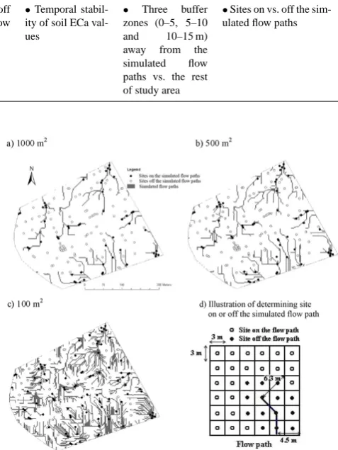
29 Figure 2. Simulated concentrated lateral flow paths at the soil–bedrock interface using three thresholds of contribution area: (a) 1,000 m2_{, (b) 500 m}2_{, and (c) 100 m}2_{. An illustration of} determining whether a soil moisture monitoring site is on or off the simulated flow path is shown in (d) (see the text for details).

Fig. 2. Simulated concentrated lateral flow paths at the soil-bedrock

interface using three thresholds of contribution area: (a) 1000 m2,

(b) 500 m2, and (c) 100 m2. An illustration of determining whether a soil moisture monitoring site is on or off the simulated flow path is shown in (d) (see the text for details).

it was considered as off the flow path. Details about deter-mining whether a site is on or off the simulated flow path are illustrated in Fig. 2d. Gish et al. (2005) used a similar crite-ria (<5 m away from the simulated flow path) to determine whether a cell was on or off predicted lateral flow paths. 2.3 Data collections for validating simulated flow paths Three sets of data were collected in the field to validate the simulated flow paths. These were: (1) soil moisture monitor-ing (includmonitor-ing volumetric soil water content and matric po-tential), (2) EMI surveys, and (3) observable soil Mn content at the three interfaces (Table 2).

30 Figure 3. Examples of fitted soil water retention curves using the model of van Genuchten (1980) for (a) Ap (silty clay loam), (b) Bt1 (silty clay), (c) Bt2 (silty clay) horizons of an Opequon series (site #9), (d) Ap (silt loam), (e) Bt1 (silty clay loam), (f) Bt2 (silty clay) horizons of a Hagerstown series (site #85), (g) Ap (silt loam), (h) Bt1 (silt loam), and (i) Bt2 (silt loam) horizons of a Murrill series (site #65).

Fig. 3. Examples of fitted soil water retention curves using the model of van Genuchten (1980) for (a) Ap (silty clay loam), (b) Bt1 (silty

clay), (c) Bt2 (silty clay) horizons of an Opequon series (site #9), (d) Ap (silt loam), (e) Bt1 (silty clay loam), (f) Bt2 (silty clay) horizons of a Hagerstown series (site #85), (g) Ap (silt loam), (h) Bt1 (silt loam), and (i) Bt2 (silt loam) horizons of a Murrill series (site #65).

Soil water content at multiple depths was monitored at 145 locations distributed throughout the study area (Fig. 1). Our procedure followed that of Lin et al. (2006). Briefly, a portable TRIME-FM Time Domain Reflectomery (TDR) Tube Probe (IMKO, Ettlingen, Germany) was used to de-termine volumetric soil water content while being placed at specific depth interval in a PVC access tube installed at each site. Readings were taken at six depth intervals of 0–0.2, 0.1–0.3, 0.3–0.5, 0.5–0.7, 0.7–0.9, and 0.9–1.1 m (represent-ing soil water content at 0.1, 0.2, 0.4, 0.6, 0.8, and 1.0 m depth, respectively). If the depth to bedrock at a monitoring site was not sufficiently deep to allow all six depth measure-ments, fewer readings were taken. For example, the actual numbers of subsoil water content observations were 110 and 96 for the 0.3–0.5 m and 0.7–0.9 m depth intervals, respec-tively. Entire study area’s soil water content at these 145 sites was collected for 12 times from 2005 to 2007 (Table 3). Seventy-four out of these 145 monitoring sites also had tensiometers installed (Fig. 1). These 74 locations were se-lected based on landforms and soil series in the study area (Table 1). Nested tensiometers were installed at five depths of 0.1, 0.2, 0.4, 0.8, and 1.0 m at each of these 74 sites. They

were 0.15 m away from the TDR access tubes. Soil matric potentials along with soil water contents at these 74 locations were measured for 14 times from 2006 to 2008 (Table 3).

Seventy out of these 145 soil cores were selected for pro-file description (Fig. 1), including the quantity and size of visible pores, roots, and Mn mottles in each horizon (includ-ing that at the three interfaces). These morphological fea-tures were estimated visually following the standard soil sur-vey procedures (Soil Sursur-vey Division Staff, 1993).

Table 3. The time table of soil water content and matric potential data collections in this study.

Soil Moisture Moni-toring

2005 2006 2007 2008

Whole area soil wa-ter content only (145 sites)

– Total 12 times

17 May, 15 June, 10 and 18 July, 3 August, and 14 October

20 and 21 June 13 and 29 March, 20 April, and 15 May

None

Soil water content and matric potential to-gether (76 sites) – Total 14 times

None 20, 21, and 30 June,

3 and 11 July

5 and 29 June, 15 July, 31 October

12, 19, and 26 June, 3 and 10 July

changing factor, all EMI readings were corrected to a stan-dard temperature of 25◦_{C. Ordinary kriging was used to} gen-erate the ECa maps for the entire study area based on its spa-tial structure (Kravchenko, 2003; Zhu and Lin, 2009). 2.4 Data analysis

For the 74 sites with both soil water content and matric po-tential measurements, soil water retention curves (SWRC) at different depths in each site were fitted with the model of van Genuchten (1980):

θ (h)−θr

θs−θr =

₁

1+(αh)n

(n−1)/n

, (1)

whereαandnare empirical parameters;θs andθr are

sat-uration and residual water contents, respectively;his matric potential andθ(h) is volumetric water content underh. Ex-amples of fitted SWRC for typical soil series, texture classes, and horizons in the study area are shown in Fig. 3. Tex-ture class was one of the main factors affecting the shape of the SWRC. For example, in the Ap horizon, as the texture class changed from silty clay loam to silt loam,θsdecreased from 0.43 to 0.37 m3m−3_{(Fig. 3a, d, g). For the same}

tex-ture class (e.g., silt loam) and soil series (e.g., the Murrill),

θs decreased from 0.37 to 0.32 m3m−3as the soil horizon

changed from Ap to Bt2 (Fig. 3g, h, i). Because of plowing and root growth, surface soils had lower bulk density, more pore space, and thus greaterθs than subsurface soils.

Volumetric soil water contents at the field capacity (0.33 kPa) and saturation (0 kPa) for each depth and each site were estimated through the fitted curve. The estimated wa-ter contents at field capacity ranged from 0.2 to 0.3 m3m−3, while the estimated water contents at saturation ranged from 0.35 to 0.45 m3m−3 for the entire study area. The ratio of field capacity over saturation ranged from 0.60 to 0.65 (with a mean of 0.63). These estimated soil water contents at field capacity and saturation of all depths and all 74 sites were grouped according to their soil horizons (Ap, Bt1, and Bt2)

31 Figure 4. Average volumetric soil water contents and their standard deviations at field capacity and saturation based on field observed soil water content and matrix potential for different textural classes and soil horizons in the study area.

Fig. 4. Average volumetric soil water contents and their standard

deviations at field capacity and saturation based on field observed soil water content and matrix potential for different textural classes and soil horizons in the study area.

and textural classes (silt loam, silty clay loam, and silty clay) (Fig. 4). The difference between Ap1 and Ap2 horizons was not considered here for two reasons: (1) the Ap1 horizon varied in thickness from 0.08 to 0.13-m in the study area; therefore, tensiometers installed at 0.1-m depth were located in the transition zones of Ap1 to Ap2 horizons; and (2) the TRIME-FM TDR probe was 0.18-m long, thus soil water content of the Ap1 (0–0.1 m below the ground surface) and Ap2 (0.1–0.3 m) could not be clearly separated. Although the Ap2 horizon was denser than the Ap1 horizon, such den-sity contrast was less strong as compared to that between Ap and Bt horizons in our study area.

For volumetric soil water content collected at each specific depth of each monitoring site, relative degree of saturation (RS) was calculated by dividing volumetric soil water con-tent by the estimated saturated water concon-tent of this horizon and textural class (Fig. 4). A RS close to 1 suggests near saturation. At a specific soil horizon interface, 95% confi-dence intervals for the RS values between sites on and off the simulated flow paths were calculated using SAS (SAS Insti-tute Inc., Cary, NC, USA). These confidence intervals were then compared using one-way ANOVA to determine whether significant differences in the RS existed between sites on

and off the simulated flow paths (Table 2). Similarly, 95% confidence intervals of the RS values at, below, and above a specific interface (Ap1–Ap2, clay layer, or soil-bedrock) were also compared to determine whether significant statis-tical differences existed (Table 2).

At each interface, temporal stability of the RS values of all 145 monitoring sites was analyzed using the approach pro-posed by Vachaud et al. (1985):

Rj =

1

N N

X

i=1

Rij, (2)

δi = 1

M M

X

j=1

(Rij −Rj Rj

), (3)

Sδ= v u u t 1

M M

X

j=1

δi_j −δi2, (4)

whereRj is the arithmetic mean of RS at all sites in dayj; Rij is the RS of a particular interface at sitei in dayj; N

is the number of monitoring sites (in this study,N= 145);δi

is the arithmetic mean of the relative difference of RS at site

i;Mis the number of times that the whole study area’s soil water content was measured (in this study,M= 12); andSδis the standard deviation ofδi. Positive or negativeδi suggests that at a particular interface, siteiis wetter or dryer, respec-tively, than the average condition of the entire study area. TheSδdepicts the magnitude of temporal stability of RS at

a particular interface at sitei. HigherSδ indicates a more

dynamic change (i.e., temporally unstable) in soil moisture. Temporal stability of the RS values between sites on and off the simulated flow paths was also compared at each interface (Table 2)

Following the same procedure, we conducted the temporal stability analysis of ECa values collected from four EMI sur-veys. Temporal stability of ECa in the three buffer zones (0– 5, 5–10, and 10–15 m away from the simulated flow paths) and the rest of the study area were statistically compared with each other through t-test in SAS (p<0.05) (Table 2). The temporal changes in ECa reflected the change in soil water content. Therefore, the magnitude of ECa temporal stability can represent the degree of change in soil water storage in the three buffer zones of the predicted flow paths vs. the rest of the study area.

At the three interfaces, Mn contents estimated from soil cores were also statistically compared between sites on and off the simulated paths through t-test in SAS (p<0.05) (Ta-ble 2). The Mn mass observed in the soil is an indicator of soil water movement as demonstrated in other studies (e.g., McDaniel et al., 2008; Walker and Lin, 2008).

3 Results

3.1 Simulated subsurface flow paths

The spatial patterns of potential lateral flow paths at the three interfaces simulated with different thresholds of contributing area (i.e., 100, 500, and 1000 m2) are illustrated in Fig. 2a–c for the soil-bedrock interface, where the patterns using the thresholds of 1000 and 500 m2were close to each other but quite different from that using the threshold of 100 m2. Be-cause of the topography of the study area, very few loca-tions (<8% of the entire area) had a contribution area>500 m2. Therefore, the simulated flow paths using the thresh-old contribution areas of 1000 and 500 m2 were sparse and similar. In comparison, 25% cells of the entire study area had contribution area>100 m2. In the subsequent analysis, we focus on comparing the simulated flow paths obtained with 500 and 100 m2thresholds. In Fig. 2a–c, water moved laterally across the landscape through the soil-bedrock inter-face in three main areas: the north-east corner, the mid-west depressional area, and the mid-south portion. When using a smaller threshold (100 m2), more areas participated in the flow, leading to 61% of the soil water monitoring sites (to-tal 88 sites) being identified as on the simulated flow paths (Fig. 2c). In contrast, during drier conditions using a larger threshold of 500 m2, only 35% of the 145 monitoring sites were identified as on the simulated flow paths (Fig. 2b). 3.2 Validating the simulated flow paths through soil

hy-drologic monitoring

At each of the three interfaces, the RS values between the monitoring sites on and off the simulated flow paths were statistically compared (Table 2). In relatively dry conditions (average volumetric soil water content −θ at the interfaces with the clay layer or bedrock was smaller than 0.28 and 0.31 m3m−3, respectively), the RS values of the sites on the simulated flow paths (500 m2 threshold) were significantly greater (p<0.05) than those sites off the paths (Fig. 5b, c). However, this was not the case at the Ap1–Ap2 inter-face (Fig. 5a). In relatively wet conditions (

−

θ > 0.28 and 0.31 m3m−3at the interfaces with the clay layer or bedrock, respectively), significant difference (p<0.05) in the RS val-ues also existed between the sites on and off the simulated flow paths (100 m2threshold) at the interfaces with the clay layer or bedrock (Fig. 5b, c), but not at the Ap1–Ap2 inter-face (Fig. 5a).

32

Figure 5. Comparison of the means and 95% confidence intervals of relative saturation (

RS

) at

the monitoring sites on and off the simulated flow paths with thresholds of 500 m

and 100 m

for (a) the Ap1–Ap2 interface, (b) the clay layer interface, and (c) the soil–bedrock interface.

Dash lines separate the relatively dry and wet conditions. Bars labeled with asterisks (*)

indicate statistically significant difference at

p

<0.05 level between sites on and off the

simulated paths.

Fig. 5. Comparison of the means and 95% confidence intervals of relative saturation (RS) at the monitoring sites on and off the simulated flow

paths with thresholds of 500 m2and 100 m2for (a) the Ap1–Ap2 interface, (b) the clay layer interface, and (c) the soil-bedrock interface. Dash lines separate the relatively dry and wet conditions. Bars labeled with asterisks (*) indicate statistically significant difference atp<0.05 level between sites on and off the simulated paths.

relatively wet conditions ( −

θ >0.28 m3m−3), such significant difference (p<0.05) in the RS values also existed between the sites on and off the flow paths simulated with the thresh-old of 100 m2_{. For the sites off the simulated flow paths,}

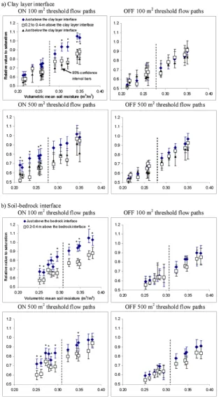
dif-ferences in the RS values between the clay layer interface and that above or below the interface were not significant under either dry or wet conditions (Fig. 6a).

For sites on the flow paths simulated with the threshold of 100 m2, the RS values at the soil-bedrock interface were significantly greater (p<0.05) than those 0.2-m above it, re-gardless of the wetness condition (Fig. 6b). In compari-son, for sites on the flow paths simulated with the threshold 500 m2, significant difference in the RS values between the soil-bedrock interface and 0.2-m above it could only be ob-served in relatively dry conditions (θ <− 0.31 m3m−3).

33 Figure 6. Comparison of the means and 95% confidence intervals of the relative saturation (RS) at the monitoring sites on and off the simulated flow paths with thresholds of 500 m2 _and 100 m2 for (a) the interface with the clay layer and (b) the interface with the bedrock. Within each graph, the comparison is for RS just above or below the specified interface and 0.2 m above the interface. Dash lines separate the relatively dry and wet conditions. Bars labeled with asterisks (*) indicate statistically significant difference at p<0.05 level.

Figure 6. Continued.

Fig. 6. Comparison of the means and 95% confidence intervals of the relative saturation (RS) at the monitoring sites on and off the simulated

flow paths with thresholds of 500 m2and 100 m2for (a) the interface with the clay layer and (b) the interface with the bedrock. Within each graph, the comparison is for RS just above or below the specified interface and 0.2 m above the interface. Dash lines separate the relatively dry and wet conditions. Bars labeled with asterisks (*) indicate statistically significant difference atp<0.05 level.

35

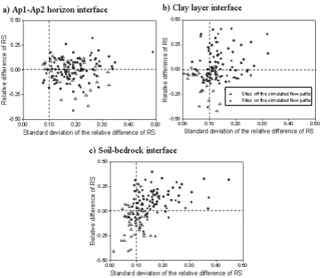
Figure 7. Temporal stability of relative saturation (RS) at the monitoring sites on and off the simulated flow paths (using the threshold of 100 m2_{) at (a) the Ap1–Ap2 interface, (b) the}

clay layer interface, and (c) the soil–bedrock interface. Sites with positive relative difference were wetter than the overall average of the entire study area. Sites with high standard deviations of the relative difference were temporally unstable (i.e., more dynamic).

Fig. 7. Temporal stability of relative saturation (RS) at the

monitor-ing sites on and off the simulated flow paths (usmonitor-ing the threshold of 100 m2) at (a) the Ap1–Ap2 interface, (b) the clay layer interface, and (c) the soil-bedrock interface. Sites with positive relative differ-ence were wetter than the overall average of the entire study area. Sites with high standard deviations of the relative difference were temporally unstable (i.e., more dynamic).

The temporal stability of the RS values between the sites on and off the simulated flow paths (100 m2) at all three interfaces were compared in Fig. 7. At the clay layer and soil-bedrock interfaces, sites on the simulated flow paths had greater relative differences of RS and standard deviations than the sites off the flow paths (Fig. 7b, c), suggesting a more dynamic (and thus unstable) moisture status over time for the sites on the flow paths. At the clay layer interface, 70% of the sites on the flow paths hadδi>0 and 75% of them

had standard deviation ofδi>0.1, while only 13% and 36%

of the sites off the flow paths hadδi>0 and standard

devi-ation ofδi>0.1, respectively. At the soil-bedrock interface,

percentages of the sites on the flow paths with positiveδi

value and high standard deviation (>0.1) were even greater, 85% and 90%, respectively, while the corresponding percent-ages were only 12% and 36% for the sites off the flow paths. At the Ap1–Ap2 interface, the sites on and off the simulated flow paths had no distinct differences inδi (Fig. 7a). When the flow path threshold was changed to 500 m2, results simi-lar to that shown in Fig. 7 were observed (data not shown). 3.3 Validating the simulated flow paths through

re-peated EMI surveys

The temporal stability of ECa values in different buffer zones of the simulated flow paths is shown in Fig. 8, with a thresh-old of 500 m2. As the distance from the simulated flow paths increased, both the mean and standard deviation of the rel-ative difference in ECa decreased, suggesting that the soils

36 Figure 8. Temporal stability of apparent electrical conductivity (ECa) in areas with different distances away from the simulated flow paths (using the threshold of 500 m2_{). Areas with}

positive relative difference in ECa indicate a higher ECa value than the overall mean of the entire study area. Areas with high standard deviation of the relative difference in ECa indicate temporally more dynamic (or unstable). Bars with the same letter are not statistically significantly different from each other at p<0.05 level.

Fig. 8. Temporal stability of apparent electrical conductivity (ECa)

in areas with different distances away from the simulated flow paths (using the threshold of 500 m2). Areas with positive relative differ-ence in ECa indicate a higher ECa value than the overall mean of the entire study area. Areas with high standard deviation of the relative difference in ECa indicate temporally more dynamic (or unstable). Bars with the same letter are not statistically significantly different from each other atp<0.05 level.

closer to the simulated flow paths tended to have elevated and more dynamic ECa values. Additionally, the positive relative differences in ECa in the three buffer zones (0–5, 5– 10, and 10–15 m) imply that their ECa values were greater than the overall average of the entire landscape. The greater standard deviations further suggest that the soil ECa values in areas closer to the simulated flow paths had higher tem-poral variations than the soils further away from these flow paths (Fig. 8).

3.4 Validating the simulated flow paths through soil Mn distribution

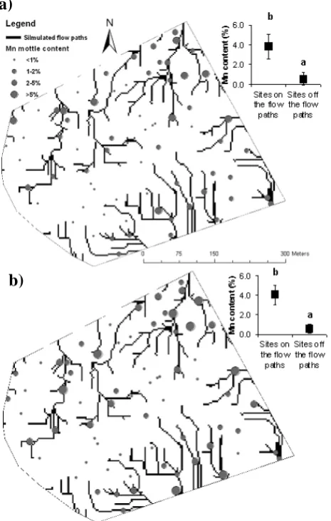
The simulated flow paths were further validated through the spatial variation in soil Mn contents at the clay layer and soil-bedrock interfaces (Table 2 and Fig. 9). For the sites on the simulated flow paths (threshold of 500 m2), soils Mn content at these two interfaces were generally greater than 1% and reached as high as 5–10% at some locations. For the sites off the simulated flow paths, almost no Mn was observed at these two interfaces. Therefore, locations with greater soil Mn content are expected to be on or closer to subsurface flow paths in the landscape studied.

4 Discussion

Our hydrological monitoring suggested that concentrated lat-eral flow paths at the interfaces with the clay layer or the bedrock were reasonably simulated with the D8 algorithm. First, soils on the simulated flow paths at these two interfaces were closer to saturation than those off the paths (Fig. 5b, c).

Figure 9. Observed Mn contents in the soil profiles at (a) the clay layer interface and (b) the

soil–bedrock interface in relation to the simulated concentrated flow paths (using a threshold

of 500 m

). In the insets, Mn contents on and off the simulated flow paths are compared. Bars

with different letters are statistically significantly different at

p

<0.05 level.

a)

b)

Fig. 9. Observed Mn contents in the soil profiles at (a) the clay

layer interface and (b) the soil-bedrock interface in relation to the simulated concentrated flow paths (using a threshold of 500 m2). In the insets, Mn contents on and off the simulated flow paths are compared. Bars with different letters are statistically significantly different atp<0.05 level.

Second, for sites on the simulated flow paths, soils at these two interfaces were also closer to saturation than soils below or above these interfaces (Fig. 6). Third, the temporal stabil-ity analysis indicated that the interfaces with the clay layer or the bedrock on the simulated flow paths were generally wet-ter and temporally less stable (Fig. 7b, c), implying generally more water movement through these interfaces. De Lannoy et al. (2006) also documented that concentrated subsurface lateral flow resulted in high temporal variability of soil water content at the clay layer interface.

Our hydrological monitoring also indicated that lateral subsurface flow did not exist at the Ap1–Ap2 interface. No significant difference in the RS values was observed between the sites on and off the simulated flow paths at the Ap1– Ap2 interface (Fig. 5a). In addition, the temporal stability

between sites on and off the simulated flow paths had no dis-tinct differences at this interface (Fig. 7a). The interfaces of different soil horizons can trigger lateral subsurface flow as reported in some previous studies (e.g., Kung, 1990, 1993; Ju and Kung, 1993; Gish et al., 2005). However, as shown in this study, not all interfaces are effective in generating lat-eral subsurface water flow in agricultural landscapes. When describing soil cores in this study, we noticed that the sur-face horizons (e.g., Ap1 and Ap2) were biologically active and had many macrospores (earthworm holes and root chan-nels). These macrospores could have transported water from the Ap1 to Ap2 horizon without much restriction during wet periods and thus prevented water from accumulating at the Ap1-Ap2 interface. Another possible reason for the lack of lateral flow between the Ap1 and Ap2 horizons was the pos-sible limitation of the monitoring devices used to determine soil moisture in these two horizons (i.e., the 0.18-m long TDR probe overlapped the Ap1 and Ap2 horizons’ readings and some tensiometers were located in the transition zones between the Ap1 to Ap2 horizons). In comparison, clay-enriched argillic horizon or dense fragipan have been widely recognized as important lateral flow paths in subsoils (e.g., Heppell et al., 2000; Gish et al., 2005; Lin et al., 2008). The clay layer interface was generally deeper than 0.4 m in our study area. At such depth, fewer macrospores were ob-served and thus the vertical water percolation could be more restricted.

The repeated EMI surveys suggested that the spatial pat-tern of subsurface lateral flow paths simulated with GIS was reasonable and compared favorably with the ECa data. We assumed that the change in soil water content was the main control of the temporal variation in ECa values during our repeated EMI surveys from January to June 2008 (note that all temperatures were corrected to a standard value). This is consistent with some previous studies that reported strong correlation between soil ECa and soil water storage (e.g., Sherlock and McDonnell, 2003; Reedy and Scalon, 2003). Thus, the higher and less stable ECa values in areas closer to the simulated flow paths (Fig. 8) suggest that the wetness there was increased and moisture dynamics was more sig-nificant. However, because we used approximately 8-m line spacing in our EMI surveys, specific subsurface lateral flow paths could not be clearly identified on the EMI maps. To do so would require a denser line spacing (e.g.,≤1 m) and per-haps also shorter time intervals (e.g., right before and after a large rainstorm) for repeating EMI surveys.

at the interfaces with the clay layer and the bedrock on the simulated flow paths, whereas soil Mn content off the simu-lated flow paths was almost zero (Fig. 9).

During the relatively dry period, more drainage areas were required to initiate the lateral subsurface flow upon rainfall inputs. Thus, a larger threshold (e.g., 500 m2) simulated better potential lateral flow paths at the clay layer interface (Fig. 5b). In contrast, during the wet period, a smaller thresh-old (e.g., 100 m2) was better to simulate potential lateral flow paths at this interface (Fig. 5b). In our study area, the soil wa-ter content generally increased with depth and often reached the highest value at the soil-bedrock interface. Even during relatively dry period, the soil at the soil-bedrock interface might still be wet and free water lateral movement could oc-cur after large rainstorms. In such case, a smaller threshold of 100 m2 could still reasonably simulate concentrated lat-eral subsurface flow paths at the soil-bedrock interface. This is supported by significant differences in the RS between the sites on and off the simulated flow paths (threshold 100 m2) during the dry period, as shown in Fig. 5c. In addition, sig-nificant differences between soil water content at the soil-bedrock interface and 0.2 m above it can also be observed for sites on the simulated flow paths (threshold 100 m2) during the dry period (Fig. 6b). This further suggests that a smaller threshold (100 m2) works better to simulate flow paths at the soil-bedrock interface under both dry and wet conditions.

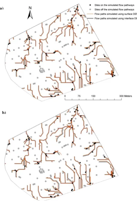
It is interesting to note that the flow paths simulated with the DEMs of the subsurface interfaces and the DEM of the land surface were nearly identical in this study, with over 90% of the simulated flow paths being the same (Fig. 10). This suggested that the flow path simulations were not im-proved much with the consideration of the subsurface inter-face DEMs in this particular landscape. This was attributed to two reasons: First, the topography of the interfaces was dominated by the variation in land surface elevation. In our study area, the maximum difference in surface elevation was 23 m between the lowest point in the footslope and the high-est point at the ridge top. However, the larghigh-est differences in the Ap1 horizon thickness and the depth to the clay layer or the bedrock for the entire landscape were less than 2 m (i.e.,

<8.7% of the surface elevation change). Second, the fine scale variation of Ap1 horizon thickness and the depth to the clay layer or the bedrock might not have been well captured through our 145 or less point-based observations and their spatial interpolations over the entire landscape of 19.5-ha in size. Similar finding was reported by Birkhead et al. (1996), in which the bedrock topography derived from GPR image was shown to be closely related to the surface topography (elevations of bedrock and ground surface decreased simul-taneously for about 1.5 m in a 90-m transect).

However, other studies observed that the topography of subsurface interfaces could be quite different from that of land surface and thus simulation based on subsurface inter-face topography would yield better results. For example, Freer et al. (2002) found that terrain attributes of land

sur-38 Figure 10. Comparison of concentrated flow paths simulated using surface DEM with those using a) the clay layer interface DEM and b) the soil-bedrock interface DEM. The threshold used in this figure is 500 m2_.

a)

b)

Fig. 10. Comparison of concentrated flow paths simulated using

surface DEM with those using (a) the clay layer interface DEM and (b) the soil-bedrock interface DEM. The threshold used in this figure is 500 m2.

face did not capture their observed spatial patterns of hills-lope (30×60 m and 34◦average slope) hydrologic response, while bedrock surface topography significantly improved the interpretation of flow spatial variation. Burns et al. (1998) documented that accumulated area simulated with bedrock surface DEM explained better the base cation concentrations in the subsurface flow along a 20×50-m hillslope. These studies have a common feature, that is, intensive depth to bedrock surveys were made in a comparatively small area (e.g.,>180 observations within an area of<0.2 ha). Thus, fine-scale variation in depth to bedrock was reasonably ob-tained in these studies.

Consequently, for areas where subsurface interface topog-raphy is dominated by surface DEM (e.g., our study area), surface DEM can be sufficiently used to simulate the sub-surface concentrated lateral flow paths. Otherwise, simula-tion based on subsurface interface DEM is more desirable. Hence, it is important to find ways to predict depth to sub-surface water-restricting layers (such as the clay layer or the bedrock) so that the cost-effectiveness of the GIS modeling could be better realized.

5 Conclusions

Through validation by soil hydrologic monitoring, EMI sur-veys, and soil morphological observations, it was apparent that concentrated subsurface lateral flow occurred at the in-terfaces with the clay layer (or water-restrictive layer) and the underlying bedrock in the agricultural landscape studied, but not at the interface between the surface plowed layers of Ap1 and Ap2 horizons (because of considerable biological activities at that interface and/or the likely limitation of the monitoring devices for clearly separating these two horizons’ soil moisture dynamics). The ArcGIS hydrologic modeling (the D8 algorithm) did a reasonable job in simulating poten-tial concentrated lateral flow paths at the interfaces in soil profiles. Such simulated subsurface lateral flow paths were temporally dynamic as they varied with the wetness condi-tion of the landscape. Hence, using different thresholds of contributing area for the GIS hydrologic simulation would be needed to obtain expected results under different mois-ture conditions (e.g., 500 m2for relatively dry conditions and 100 m2for relatively wet conditions in this study). A suffi-ciently detailed DEM is also needed to ensure that the GIS flow algorithm performs with lower uncertainty. We suggest additional testing of this cost-effective means of predicting likely subsurface concentrated flow paths in other landscapes in order to establish a solid protocol for simulating subsur-face hydrologic flow paths in different watersheds. However, some costs would incur in obtaining necessary data for such simulation to be effective, mainly in areas where subsurface interface topography differs significantly from land surface topography. Thus, finding means of predicting depth to sub-surface water-restricting layers (such as the clay layer or the bedrock) will enhance the cost-effectiveness of the GIS mod-eling. In areas where subsurface interface topography does vary similarly with surface topography, surface DEM can be used to approximate subsurface interface topography to obtain similar results. Repeated EMI surveys provide an-other low-cost and nondestructive means of detecting poten-tial concentrated subsurface flow paths; however, dense sam-ple spacing and frequently repeated surveys would be needed if specific subsurface flow paths are to be identified via re-peated EMI surveys. While soil morphological features such as Mn distribution in soil profiles also serve as useful simple indicators of subsurface water flow paths, it does require soil sampling (by excavation or augering) with sufficient num-bers of observations to possibly infer landscape-scale sub-surface flow paths.

Acknowledgements. This research was partially supported by the

USDA Higher Education Challenge Competitive Grants Program (Grant no. 2006-38411-17202).

Edited by: J. Seibert

References

Auerswald, K., Simon, S., and Stanjek, H.: Influence of soil proper-ties on electrical conductivity under humid water regimes, Soil. Sci., 166, 382–390, 2001.

Bakhsh, A. and Kanwar, R. S.: Soil and landscape attributes inter-pret subsurface drainage clusters, Aust. J. Soil. Res., 46, 735– 744, 2008.

Birkhead, A. L., Heritage, G. L., White, H., and van Niekerk, A. W.: Ground-penetrating radar as a tool for mapping the phreatic surface, bedrock profile, and alluvial stratigraphy in the Sabie River, Kruger National Park, J. Soil Water Cons., 51, 234–241, 1996.

Bogaart, P. W. and Troch, P. A.: Curvature distribution within hillslopes and catchments and its effect on the hydrological re-sponse, Hydrol. Earth Syst. Sci., 10, 925–936, 2006,

http://www.hydrol-earth-syst-sci.net/10/925/2006/.

Burns, D. A., Hooper, R. P., McDonnell, J. J., Freer, J. E., Kendall, C., and Beven, K.: Base cation concentrations in subsurface flow from a forested hillslope: The role of flushing frequency, Water Resour. Res., 34, 3535–3544, 1998.

Buttle, J. M. and McDonald, D. J.: Coupled vertical and lateral pref-erential flow on a forested slope, Water Resour. Res., 38, 1060, doi:10.1029/2001WR000773, 2002.

Cassel, D. K., Afyuni, M. M., and Robarge, W. P.: Manganese dis-tribution and patterns of soil wetting and depletion in a piedmont hillslope, Soil Sci. Soc. Am. J., 66, 939–947, 2002.

Chen, S. K., Liu, C. W., and Huang, H. C.: Analysis of water move-ment in paddy rice fields (II) simulation studies, J. Hydrol., 268, 259–271, 2002.

Corwin, D. L. and Lesch, S. M.: Apparent soil electrical conduc-tivity measurements in agriculture, Comput. Electron. Agr., 46, 11–43, 2005.

De Lannoy, G. J. M., Verhoest, N. E. C., Houser, P. R., Gish, T. J., and van Meirvenne, M.: Spatial and temporal characteris-tics of soil moisture in an intensively monitored agricultural field (OPE3), J. Hydrol., 331, 719–730, 2006.

Elliot, J. A., Cessna, A. J., Best, K. B., Nicholaichuk, W., and Tollefson, L. C.: Leaching and preferential flow of clopyralid under irrigation: field observations and simulation modeling, J. Environ. Qual., 27, 124–131, 1998.

Erskine, R. H., Green, T. R., Ramirez, J. A., and MacDon-ald, L. H.: Comparison of gridbased algorithms for comput-ing upslope contributcomput-ing area, Water Resour. Res., 42, W09416, doi:10.1029/2005WR004648, 2006.

Fairfield, J. and Leymarie, P.: Drainage networks from grid digital elevation models, Water Resour. Res., 27, 709–717, 1991. Fiori, A., Romanelli, M., Cavalli, D. J., and Russo, D.:

Numeri-cal experiments of streamflow generation in steep catchments, J. Hydrol., 339, 183–192, 2007.

Freer, J., McDonnell, J. J, Beven, K. J., Brammer, D., Burns, D. A, Hooper, R. P., and Kendall, C.: Topographic controls on sub-surface storm flow at the hillslope-scale for two hydrologically distinct small catchments, Hydrol. Processes., 11, 1347–1352, 1997.

Freer, J., McDonnell, J. J, Beven, K. J., Peters, N. E., Burns, D. A, Hooper, R. P., Aulenbach, B., and Kendall, C.: The role of bedrock topography on subsurface storm flow, Water Resour. Res., 38, 1269, doi:10.1029/2001WR000872, 2002.

Doolittle, J. A., and Miller, P. T.: Evaluating use of ground-penetrating radar for identifying subsurface flow pathways, Soil Sci. Soc. Am. J., 66, 1620–1629, 2002.

Gish, T. J., Walthall, C. L., Daughtry, C. S. T., and Kung, K.-J. S.: Using soil moisture and spatial yield patterns to identify subsur-face flow pathways, J. Environ. Qual., 34, 274–286, 2005. Guo, J. H., Liang, X., and Leung, L. R.: A new multiscale flow

network generation scheme for land surface models, Geophys. Res. Lett., 32, L23502, doi:10.1029/2004GL021381, 2004. Haga, H., Matsumoto, Y., Matsutani, J., Fujita, M., Nishida, K.,

and Sakamoto, Y.: Flow paths, rainfall properties, and an-tecedent soil moisture controlling lags to peak discharge in a granitic unchanneled catchment, Water Resour. Res., 41, W12410, doi:10.1029/2005WR004236, 2005.

Haria, A. H., Johnson, A. C., Bell, J. P., and Batchelor, C. H.: Water-movement and isoproturon behaviour in a drained heavy clay soil. 1. Preferential flow processes, J. Hydrol., 163, 201– 216, 1994.

Heppell, C. M., Burt, T. P., and Williams, R. J.: Variations in the hy-drology of an underdrained clay hillslope, J. Hydrol., 227, 236– 256, 2000.

Jones, R.: Algorithms for using a DEM for mapping catchment areas of stream sediment samples, Comput. Geosci., 28, 1051– 1060, 2002.

Ju, S. H. and Kung, K.-J. S.: Finite element simulation of funnel flow and overall flow property induced by multiple soil layers, J. Environ. Qual., 22, 432–442, 1993.

Kenny, F., Matthews, B., and Todd, K.: Routing overland flow through sinks and flats in the interpolated raster terrain surfaces, Comput. Geosci., 34, 1417–1430, 2008.

Kettler, T. A., Doran, J. W., and Gilbert, T. L.: Simplified method for soil particle-size determination to accompany soil-quality analyses, Soil Sci. Soc. Am. J., 65, 849–852, 2001.

Kirkby, M. J.: Thresholds and instability in stream head hollows: a model of magnitude and frequency for wash processes, in: Pro-cess Models and Theoretical Geomorphology, edited by: Kirkby, M. J., Wiley, Chichester, UK, 295–314, 1994.

Kitahara, H., Terajima, T., and Nakai, Y.: Ratio of pipe flow to throughflow discharge, J. Jpn. Forest. Soc., 76, 10–17, 1994. Krovchenko, A. N.: Influence of spatial structure on accuracy of

in-terpolation methods, Soil Sci. Soc. Am. J., 67, 1564–1571, 2003. Kravchenko, A. N. and Robertson, G. P.: Can topographical and yield data substantially improve total soil carbon mapping by re-gression kriging? Agron. J., 99, 12–17, 2007.

Kung, K.-J. S.: Preferential flow in a sandy vadose zone: 1. Field observation, Geoderma, 46, 30 51–71, 1990.

Kung, K.-J. S.: Laboratory observation of the funnel flow mecha-nism and its influence on solute transport, J. Environ. Qual., 22, 91–102, 1993.

Lin, H. S., Bouma, J., Wilding, L. P., Richardson, J.L., Kutilek, M., and Nielsen, D. R.: Advances in hydropedology, Adv. Agron., 85, 1–89, 2005.

Lin, H. S., Kogelmann, W., Walker, C., and Bruns, M. A.: Soil moisture patterns in a forested catchment: A hydropedological perspective, Geoderma, 131, 345–368, 2006.

Lin, H. S., Brook, E., McDaniel, P., and Boll, J.:Hydropedology and Surface/Subsurface Runoff Processes, in: Encyclopedia of Hydrologic Sciences.edited by: Anderson, M. G., John Wiley & Sons, Ltd., doi:10.1002/0470848944.hsa306, 1–25, 2008.

Maidment, D.: Arc Hydro: GIS for Water Resources, ESRI, Red-lands, CA, USA, 55–86, 2002.

Marks, D., Dozier, J., and Frew, J.: Automated basin delineation from digital elevation data, GeoProcessing, 2, 299–311, 1984. McDaniel, P. A. and Buol, S. W.: Manganese distributions in acid

soils of the North Carolina Piedmont, Soil Sci. Soc. Am. J., 55, 152–158, 1991.

McDaniel, P. A., Regan, M. P., Brooks, E., Boll, J., Bamdt, S., Falen, A., Young, S. K., and Hammel, J. E.: Linking fragi-pans, perched water tables, and catchment-scale hydrological processes, Catena, 73, 166–173, 2008.

Noguchi, S., Tsuboyama, Y., Sidle, R. C., and Hosoda, I.: Mor-phological characteristics of macropores and the distribution of preferential flow paths in a forested slope segment, Soil Sci. Soc. Am. J., 63, 1413–1423, 1999.

O’Callaghan, J. F. and Mark, D. M.: The extraction of drainage networks from digital elevation data, CVGIP, 28, 323–344. 1984. Orlandini, S., Moretti, G., Franchini, M., Aldighieri, B., and Testa, B.: Path-based methods for the determination of nondispersive drainage directions in grid-based digital elevation models, Water Resour. Res., 39, 1144, doi:10.1029/2002WR001639, 2003. Paik, K.: Global search algorithm for nondispersive

flow path extraction, J. Geophys. Res., 113, F04001, doi:10.1029/2007JF000964, 2008.

Palkovics, W. E. and Petersen, G. W.: Contribution of lateral soil-water movement above a fragipan to streamflow, Soil Sci. Soc. Am. J., 41, 394–400, 1977.

Patrick, W. H. and Henderson, R. E.: Reduction and reoxidation cy-cles of Manganese and Iron in flooded soil and in water solution, Soil Sci. Soc. Am. J., 45, 855–859, 1981.

Perillo, C. A., Gupta, S. C., and Moncrief, J. F.: Prevalence and initiation of preferential flow paths in a sandy loam with argillic horizon, Geoderma, 89, 307–331, 1999.

Quinn, P. F., Beven, K. J., Chevallier, P., and Planchon, O.: The prediction of hillslope flowpaths for distributed modelling using digital terrain models, Hydrol. Proc., 5, 59–80, 1991.

Reedy, R. C. and Scanlon, B. R.: Soil water content monitoring using electromagnetic induction, J. Geotech. Geoenviron. Eng., 129, 1028–1039, 2003.

Rhoades, J. D., Raats, P. A. C., and Prather, R. S.: Effects of liquid-phase electrical conductivity water content and surface conduc-tivity on bulk soil electrical conducconduc-tivity, Soil Sci. Soc. Am. J., 40, 651–665, 1976.

Sander, T. and Gerke, H. H.: Preferential flow patterns in paddy fields using a dye tracer, Vadose Zone. J., 6, 105–115, 2007. Seibert, J. and McGlynn, B. L.: A new triangular multiple flow

direction algorithm for computing upslope areas from grid-ded digital elevation models, Water Resour. Res., 43, W04501, doi:10.1029/2006WR005128, 2007.

Sch¨auble, H., Marinoni, O., and Hinderer, M.: A GIS-based method to calculate flow accumulation by considering dams and their specific operation time, Comput. Geosci., 34, 635–646, 2008. Sherlock, M. D. and McDonnell, J. J.: A new too for hillslope

hydrologists: spatial distributed groundwater level and soilwa-ter content measured using electromagnetic induction, Hydrol. Proc., 17, 1965–1977, 2003.

Sidle, R. C., Noguchi, S., Tsuboyama, Y., and Laursen, K.: A conceptual model of preferential flow systems in forested hill-slopes: evidence of self-organization, Hydrol. Proc., 15, 1675–

1962, 2001.

Soil Survey Division Staff.: Soil Survey Manual, U.S. Department of Agriculture Handbook No. 18, US Government Printing Of-fice, Washington, DC, USA, 1993.

Sørensen, R., Zinko, U., and Seibert, J.: On the calculation of the topographic wetness index: evaluation of different methods based on field observations, Hydrol. Earth Syst. Sci, 10, 101– 112, 2006.

Tarboton, D. G.: A new method for the determination of flow direc-tions and upslope areas in grid digital elevation models, Water Resour. Res., 33, 309–319, 1997.

Thompson, J. A., Pena-Yewtukhiw, E. M., and Grove, J. H.: Soil-landscape modelling across a physiographic region: Topo-graphic patterns and model transportability, Geoderma, 133, 57– 70, 2006.

Tsukamoto Y. and Ohta, T.: Runoff process on a steep forested slope, J. Hydrol., 102, 165–178, 1988.

Vachaud, G., De Silans Passerat, A., Balabanis, P., and Vauclin, M.: Temporal stability of spatial measured soil water probability density function, Soil Sci. Soc. Am. J., 49, 822–827, 1985. Van Genuchten, M. T.: A closed form equation for predicting the

hydraulic conductivity of unsaturated soils, Soil Sci. Soc. Am. J., 44, 892–898, 1980.

Vogt, J. V., Colombo, R., and Bertolo, F.: Deriving drainage net-works and catchment boundaries: a new methodology combin-ing digital elevation data and environmental characteristics, Ge-omorphology, 53, 281–298, 2003.

Walker, C. and Lin, H. S.: Soil property changes after four decades of wastewater irrigation: a landscape perspective, Catena, 73, 63–74, 2008.

Wu, S., Li, J., and Huang, G. H.: A study on DEM-derived primary topographic attributes for hydrologic applications: sensitivity to elevation data resolution, Appl. Geogr., 28, 210–223, 2008. Yaalon, D. H., Jungreis, C., and Koyumjisky, H.: Distribution and

reorganization of manganese in three catenas of Mediterranean soils, Geoderma, 7, 71–78, 1972.

Zhu, Q. and Lin, H. S.: Combining sample size, spatial structure, and auxiliary variables to determine optimal kriging in contrast-ing landscapes, Ecol. Model., in review, 2009.

Zhu, Q., Lin, H. S., and Doolittle, J.: Repeated electromagnetic in-duction surveys for understanding landscape soil and water dy-namics, Soil Sci. Soc. Am. J. in review, 2009.