www.hydrol-earth-syst-sci.net/14/603/2010/ © Author(s) 2010. This work is distributed under the Creative Commons Attribution 3.0 License.
Earth System
Sciences
An experiment on the evolution of an ensemble of neural networks
for streamflow forecasting
M.-A. Boucher, J.-P. Lalibert´e, and F. Anctil
Chaire de recherche EDS en pr´evisions et actions hydrologiques, D´epartement de g´enie civil, Universit´e Laval, Pavillon Pouliot, Qu´ebec, G1K 7P4, Canada
Received: 9 September 2009 – Published in Hydrol. Earth Syst. Sci. Discuss.: 6 October 2009 Revised: 9 March 2010 – Accepted: 19 March 2010 – Published: 30 March 2010
Abstract. We present an experiment on fifty multilayer per-ceptrons trained for streamflow forecasting on three water-sheds using bootstrapped input series. This type of neural network is common in hydrology and using multiple train-ing repetitions (ensembltrain-ing) is a popular practice: the infor-mation issued by the ensemble is then aggregated and con-sidered to be the final output. Some authors proposed that the ensemble could serve the calculation of confidence in-tervals around the ensemble mean. In the following, we are interested in the reliability of confidence intervals ob-tained in such fashion and in tracking the evolution of the ensemble of neural networks during the training process. For each iteration of this process, the mean of the ensem-ble is computed along with various confidence intervals. The performance of the ensemble mean is evaluated based on the mean absolute error. Since the ensemble of neural net-works resemble an ensemble streamflow forecast, we also use ensemble-specific quality assessment tools such as the Continuous Ranked Probability Score to quantify the fore-casting performance of the ensemble formed by the neural networks repetitions. We show that while the performance of the single predictor formed by the ensemble mean improves throughout the training process, the reliability of the associ-ated confidence intervals starts to decrease shortly after the initiation of this process. While there is no moment during the training where the reliability of the confidence intervals is perfect, we show that it is best after approximately 5 to 10 it-erations, depending on the basin. We also show that the Con-tinuous Ranked Probability Score and the logarithmic score do not evolve in the same fashion during the training, due to a particularity of the logarithmic score.
Correspondence to: M.-A. Boucher
1 Introduction
Neural networks are used in hydrology since the 1990’s (e.g. Kang et al., 1993; Karunanithi et al., 1994; Campolo et al., 1999; Tokar and Johnson, 1999). They have also been the object of some experiments in meteorology (e.g. Hsieh and Tang, 1998; Valverde Ram´ırez et al., 2005) and climatology (e.g. Knutti et al., 2003). Although it can be argued that neu-ral networks models cannot contribute to the understanding of the processes at hand and that they are most often over parametrized, they remain very useful as simple, rapidly im-plemented, rainfall-runoff models.
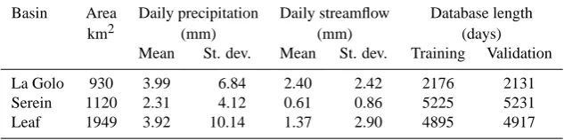
Table 1. Characteristics of the watersheds and corresponding databases used in the experiment.
Basin Area Daily precipitation Daily streamflow Database length
km2 (mm) (mm) (days)
Mean St. dev. Mean St. dev. Training Validation
La Golo 930 3.99 6.84 2.40 2.42 2176 2131
Serein 1120 2.31 4.12 0.61 0.86 5225 5231
Leaf 1949 3.92 10.14 1.37 2.90 4895 4917
provide a single final output, either by simple or weighted averaging, by a regression between ensemble members or by other more sophisticated means (e.g. Freitas and Rodrigues, 2006).
Some authors also suggested that an ensemble could be used to issue confidence intervals to be associated with the forecast (e.g. Lajbcygier and Connor, 1997; Papadopoulos and Edwards, 2001; Shrestha and Solomatine, 2006b). How-ever, it is our opinion that the reliability of such confidence intervals has rarely been investigated.
The recent development of bayesian neural networks (e.g. Mackay, 1992; Neal, 1996) and their successful applica-tion in probabilistic hydrological forecasting (e.g. Khan and Coulibaly, 2006; Kingston et al., 2005) suggest that they are the most appropriate tools to achieve reliable ensemble and probabilistic hydrological forecasting with neural networks. Nevertheless, MLPs remain very popular among hydrolo-gists for their simplicity of implementation and because they produce very accurate forecasts for a wide range of situa-tions. Therefore, it can be interesting to have a closer look at an ensemble of MLPs, as it evolves during training, and to assess the reliability of the probabilistic distribution they col-lectively form. Besides bayesian networks, there exist some other experiments regarding probabilistic-type forecasts with neural networks, such as the work by Carney et al. (2005), in which they use ensembles of Mixture Density networks to issue probabilistic surf height forecasts.
Here we propose an experiment where we follow an en-semble of MLPs during their training process, in a one-day-ahead streamflow forecasting situation. As the MLP ensem-ble evolves, we will investigate their probabilistic perfor-mance and compare it to the deterministic perforperfor-mance of a single predictor formed by averaging the individual neu-ral network outputs. We will also pay close attention to the reliability of the confidence intervals computed from the en-sembles. Because MLP ensembles resemble ensembles is-sued by an operational hydrological forecasting system, we will resort to typical ensemble-based performance assess-ment tools.
The remaining of the paper is divided as follows: the context of application is described in the next section, with a short description of the watersheds and corresponding databases. The subsequent section presents the protocol of
experiment, including the neural networks architecture, the ensemble construction methodology and the criteria used for performance evaluation. Results are presented in Sect. 4 along with a discussion on the relevant findings of this work. The paper ends with concluding remarks and perspectives at Sect. 5.
2 Context of application
2.1 The Leaf, Serein and Le Golo watersheds
The investigation described in this paper relies on databases for three watersheds with a residence time of the order of three days, representing different hydrological behaviours. A summary of the information related to them is provided in Table 1, while hydrographs are drawn in Fig. 1.
The Le Golo River is located in Corsica, France. There are many gauging stations along this river, which is the greatest of the island. The one with the longest record, located in Vol-pajola near the basin’s outlet, will be used. This mountainous basin generates on some occasions relatively high streamflow in summer, while flow is usually maximal during winter and spring (Fig. 1a). The Serein River (Fig. 1b) is an unregulated tributary of the Yonne River, which joins the Seine River upstream of Paris. It exhibits a strong seasonal cycle (see Fig. 1b). Finally, the Leaf River is located near Collins, Mis-sissippi, USA. Although this watershed also exhibits a sea-sonal cycle (see Fig. 1c), it is not very pronounced.
All data are standardized before being fed to the neural networks. This procedure ensures that all input data have the same range of values.
3 Protocol of experiment
3.1 Separation of the databases in subsets
0 50 100 150 200 250 300 350 0
2 4 6 8 10
(b)
Streamflow (mm)
0 50 100 150 200 250 300 350
0 20 40 60
(c)
Streamflow (mm)
Days
0 50 100 150 200 250 300 350
0 5 10 15 20
(a)
Streamflow (mm)
Mean Min Max Mean Min Max
[image:3.595.50.286.65.380.2]Mean Min Max
Fig. 1.Daily mean, maximum and minimum streamflows for the (a) Le Golo (b) Serein and (c) Leaf Rivers.
figure
21
Fig. 1. Daily mean, maximum and minimum streamflows for the
(a) Le Golo (b) Serein and (c) Leaf Rivers.
clusters. The observations are therefore distributed in those clusters according to their similarities. The number of output neurons (clusters) must be determined by a calibration pro-cess. Here we use the same Kohonen network as Anctil and Lauzon (2004). After testing for many configurations of the output map, they determined that a 3×3 map was optimal. Once the nine clusters are identified, two subsets of identical size are created by randomly selecting daily events within each cluster. This ensures that the training dataset is statisti-cally equivalent to the testing dataset, thus avoiding, for ex-ample, that the training set comprises many large streamflow events while the testing set contains few. A small experi-ment was also carried out where the database for each basin was split in two halves in order to maintain the chronologi-cal order in the training and rainingesting databases. Various statistics (mean, standard deviation, minimum and maximum value, kurtosis and skewness) were computed for those two datasets as well as for the training and testing datasets used in the experiment presented in this paper. Although the chrono-logically ordered datasets did not have enormous disparities in their statistics, the training and testing datasets obtained using the self organizing map were even more similar, with almost identical statistics.
The temporal correlation in the data is preserved even if the chronological order of the original series is not. All wa-tersheds used in this study have a response time of about three days. Because multilayer perceptrons (see Sect. 3.2) do not account for the temporal correlation between the in-puts and the output, it has to be recreated artificially. To achieve this, we first use the entire database, with all en-tries in chronological order, to produce an by 5 matrix,n
being the number of streamflow observations in the whole database. The fifth column is the observed streamflow. The first three columns are the observed precipitation values for the three previous days. The fourth column is the observed streamflow for the previous day. Then, the Kohonen map-ping, separation of the database and bootstrap are performed using the row indices, ensuring that the observed streamflow is accompanied by the appropriate previous data in chrono-logical order. Because the response time is limited (three days), there is no need to provide the network with observa-tions further in the past.
3.2 Basic neural network architecture
The MLPs used to conduct this study comprise three lay-ers: the input layer, the hidden layer in which there are five neurons, and the output layer in which there is only one neu-ron. The input layer is constituted of the observed streamflow (Q) at the present timetand the precipitation (P) at timest,
t−1 andt−2. The output neuron issuesQt+1, the
one-day-ahead streamflow. The number of hidden neurons and input selection follows the trial and error process performed in the work by Anctil and Lauzon (2004) on the same data sets. Each input vector is connected to each neuron in the hidden layer and each neuron in the hidden layer is connected to the output neuron. A weight value (Wi,j or Wj,k), wherei,j
andkrepresent, respectively, the input number, the neuron number and the output number is assigned to each of these links. A bias (bj) value is also assigned to each neuron of
the hidden and output layers. The weights and biases are the parameters of the neural model. They are randomly initial-ized and then an iterative optimization process is performed until the outputs of the model match the recorded observed streamflow data. Each iteration is called an “epoch” and the optimization algorithm is Levenberg-Marquardt Backpropa-gation (Levenberg, 1944; Marquardt, 1963).
The transfer function for the neurons in the hidden layer is the sigmoid tangent, given by
C(ξ )= 2
1+e−2ξ−1, (1)
whereξ represents the weighted sum of input vectors plus biasbj and is given by
ξj=PtW1,j+Pt−1W2,j+Pt−2W3,j+QtW4,j+bj. (2)
0 50 100 150 200 250 300 350 400 450 500 0.293
0.2955 0.298 0.3005 0.303 0.3055
Ensemble size (members)
[image:4.595.50.285.60.237.2]mean CRPS (mm)
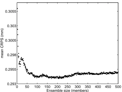
Fig. 2.Variation of the CRPS with the number of neural networks in the ensemble (Le Golo River).
22
Fig. 2. Variation of the CRPS with the number of neural networks
in the ensemble (Le Golo River).
The architecture described above is very simple, but pro-duces unbounded models. They are good interpolators, but have uncontrolled extrapolation capacities. When predict-ing streamflow, the absence of a lower limit for the forecast sometimes causes the network to issue negative values. Cre-spo et al. (1993) chose to replace those negative forecasts with zeros. In this study, we chose to replace them by the smallest archived streamflow observation for each watershed. 3.3 Ensemble construction
An ensemble formed of the outputs of 50 randomly initial-ized and individually trained MLPs was set up for every watershed: a strategy that is largely inspired from bagging (Breiman, 1996), in which each of the 50 forecasted time series is called a member of the ensemble. Therefore, the procedure asks for 50 bootstrapped training datasets (Efron and Tibshirani, 1993), a convenient way of accounting, at least to some extent, for the uncertainty component linked to the observations (e.g. Zhang et al., 2009; Ajami et al., 2007). The produced ensembles thus combine sources of uncertainty associated to the observations, through the boot-strap, and sources of uncertainty associated to the model, through a multi-model approach.
During training, the networks’ parameters are stored for each epoch in order to be able to apply the partially trained networks to the testing dataset. The latter is not used at any moment of the training process, respecting Klemeˇs (1986) split sample strategy.
The choice of producing 50 members was determined ex-perimentally. Using the databases at hand, the mean CRPS, which is explained later at Sect. 3.4, was computed for en-sembles up to 500 members. Even if the mean CRPS does continue to decrease and stabilizes at about 200, we be-lieve that fifty members are deemed sufficient to provide an
accurate estimation, as illustrated by Fig. 2. Coincidently, the ECMWF operational meteorological ensemble prediction system consists of fifty members.
The bootstrap strategy has been confronted with two other options: producing only 5 or 10 bootstrapped series, which means that each new series are used to train 10 or 5 networks, respectively. Results of this test are not reported here because no clear distinction could be identified in terms of CRPS or other score values.
3.4 Multicriteria evaluation of performance
In order to assess the performance of the ensemble at each epoch of the learning process, we used the following ensemble-specific quality evaluation tools. First, we used nu-merical criteria, namely the Continuous Ranked Probability Score (CRPS) and its corresponding decomposition (Hers-bach, 2000) as well as the logarithmic score (e.g. Good, 1952). We also used graphical quality assessment tools: the rank histogram (Talagrand et al., 1997; Hamill and Colucci, 1997) and reliability diagram (e.g. Wilks, 1995). Since these tools are described in great details in references such as Wilks (1995) and Jolliffe and Stephenson (2003), only a short description is provided hereafter.
We adopt the point of view of Gneiting and Raftery (2007), according to which a good ensemble forecast maximizes sharpness, subject to calibration. While sharpness refers to the precision of the ensemble members, calibration refers to the statistical consistency between the forecasts and the ob-servations. An ensemble forecasting system is sharp if all the members of the ensemble are close to the observed value. This ensemble forecasting system is also well calibrated (re-liable) if the dispersion of the ensemble reflects the true un-certainty of the situation.
In this view, reliability (calibration) precedes precision (sharpness) in ensemble or probabilistic forecasting since the final goal is most often expressing the forecast in terms of a probability or providing the user with a way of assessing the uncertainty on the next outcome. Therefore, however pre-cise an ensemble forecast may be, if it is not reliable it is not useful.
3.4.1 The continuous ranked probability score
LetF (x)be the cumulative distribution function (cdf) fitted
from the ensemble members,xthe predicted values at timet,
xobsthe observed value at the same time, and 1 the indicator
function. The CRPS consists in an integral of the difference between two cumulative distributions. It is defined as CRPS(F,xobs)=
1
N N
X
t=1
Z ∞ −∞
(Ft(x)−1{x≥xobs,t})2dx, (3)
for the fact that it is a comparison between a distribution and a scalar.
Gneiting and Raftery (2007) have formally demonstrated that the CRPS for probabilistic forecasts is equivalent to the mean absolute error (MAE) for single forecasts. This result is based on previous mathematical proofs by Baringhaus and Franz (2004) and by Sz´ekely and Rizzo (2005). It thus pro-vides a convenient way to compare the performance of en-semble forecasts (mean CRPS) with the performance of sin-gle forecasts (MAE) for the same watershed. Here, the MAE is calculated using the average of all members of the NN en-semble as a single forecast.
Like for the MAE, the lower the CRPS, the better it is. The lower bound is zero for both. However, the CRPS and MAE values are directly proportional to the absolute value of the observation.
An interesting characteristic of the CRPS is that it can be decomposed in two components (Hersbach, 2000).
CRPS=Rel+CRPSPot, (4)
where Rel is the reliability component and CRPSPotis the
po-tential mean CRPS. The former quantifies the extent to which the spread of the ensemble is really representative of the un-certainty associated with the forecasting situation, while the latter is the mean CRPS value that would be attained if the system was made perfectly reliable. This second component depends mostly on the data and on the choice of the model used to issue the forecasts.
This decomposition is based on the empirical cdf of the ensemble of neural networks. The two components are cal-culated with Eqs. (5 and 6)
Rel=
n
X
k=0
gk(ok−Pk)2, (5)
CRPSPot= n
X
k=0
gkok(1−ok), (6)
where Pk =n1 is the empirical cdf. The subscript k=
0,1,...,50 refers to the sorted ensemble members. gk and
ok are calculated using
gk=αk+βk (7)
and
ok=
βk
αk+βk
, (8)
whereαkandβkrepresent, respectively, the mean difference (in mm) between two forecasts in the sorted ensembles, for streamflow values inferior or superior to the observation.
3.4.2 The logarithmic score
The logarithmic score, or ignorance score (e.g. Roulston and Smith, 2002), is the logarithm of the probability density,
f (xobs), associated with the observed value. Consequently,
a gamma pdf was fitted to the ensemble of neural networks at every time step for all basins and all epochs using the maximum likelihood estimation. LetS be the score value,
f (x)the predictive distribution andxobsthe observed value.
Therefore, the value taken by the score is:
S(f (x),xobs)= −log(f (xobs)) (9)
We use the logarithmic score in the negative orientation for reasons of coherence with the MAE and the CRPS. How-ever, there is no lower bound for this score. In addition, when the observation falls outside of the predictive distri-bution, the corresponding probability density is zero. This produces an infinite value, which affects the calculation of the mean score. Here, we chose to replace those individual infinite scores by the next worst non-infinite value.
3.4.3 The rank histogram
The principle behind the rank histogram lies in the fact that if the ensemble forecasts are well calibrated, the observed value could be considered as a supplementary member of the ensemble. The construction of such a histogram is simple (Talagrand et al., 1997). The observed value at timetis first added to the corresponding forecasted ensemble and this new ensemble is sorted. For each forecast-observation pair, the rank of the observation is stored. Then, those ranks are plot-ted in a histogram. In the perfect case, this histogram is flat, so all ranks have equal relative frequency. A “U” shaped rank histogram indicates that the predictive distribution is underdispersed, so the observation falls outside the ensem-ble. Conversely, if the rank histogram has an arched form, it means that the distribution is overdispersed. If the rank his-togram is asymmetric, the observation occupies some ranks more frequently than others. It can point out a bias in the forecasts.
3.4.4 The reliability diagram
0 5 10 15 20 25 30 35 40 0
0.5 1 1.5
CRPS and MAE (mm) 0 5 10 15 20 25 30 35 400
2 4 6 (a)
Logarithmic score
0 5 10 15 20 25 30 35 40
0 0.1 0.2 0.3
CRPS and MAE (mm) 0 5 10 15 20 25 30 35 40−0.5
0 0.5
Logarithmic score
(b)
0 5 10 15 20 25 30 35 40
0 0.5 1 1.5
CRPS and MAE (mm)
CRPS MAE
0 5 10 15 20 25 30 35 400
0.5 1
Epochs
Logarithmic score
(c)
[image:6.595.50.287.63.298.2]LOG
Fig. 3.CRPS, MAE and logarithmic score as a function of the number of training epochs for (a) Le Golo,
(b) Serein, and (c) Leaf Rivers.
23
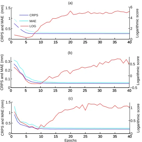
Fig. 3. CRPS, MAE and logarithmic score as a function of the
number of training epochs for (a) Le Golo, (b) Serein, and (c) Leaf Rivers.
the nominal and effective coverage values, meaning that the nominal level of confidence of each interval corresponds to the effective coverage. In addition, for two equally reliable forecasting systems, this diagram allows the user to choose the system with the best resolution, that is, the one which provides the shortest widths for confidence intervals.
Over and under dispersion problems can also be diagnosed using the reliability diagram. Overdispersion corresponds to a situation where effective coverage is greater than nominal coverage of the confidence intervals. Underdispersion corre-sponds to opposite situation.
4 Results
As explained in Sect. 3.4.1, the CRPS reduces to the absolute error in the case of a deterministic forecast, which allows the direct comparison of the performance of ensemble and de-terministic forecasts for the same watershed (e.g. Vel´azquez et al., 2009). It is common practice to generate an ensemble of neural networks and to aggregate their outputs to form a deterministic forecast. Here, the performance of this deter-ministic forecast was compared with the performance of the ensemble (not averaged) forecast. Results are shown in Fig 3, which presents the mean CRPS, MAE and mean logarithmic score calculated on the testing set. For all basins and every epoch, the CRPS values are lower than the MAE values. It indicates that the ensemble of neural networks performs bet-ter when taken as a whole than when aggregated in a single averaged predictor.
0 10 20 30 40
−2.5 −2 −1.5 −1 −0.5 0 0.5 1 1.5 2 2.5 3
Number of training epochs Neural networks individual mean error for daily streamflow forecasts (mm)
[image:6.595.309.544.65.252.2]NN1 NN2 NN3 NN4 NN5 NN6 NN7 NN8 NN9 NN10
Fig. 4.Mean error as a function of the number of training epochs for ten neural networks (le Golo River)
24
Fig. 4. Mean error as a function of the number of training epochs
for ten neural networks (Le Golo River).
As expected, because of random initialization, the first training epochs offer poor performance (Fig. 3). However, this improves rapidly over the next training epochs, before reaching a plateau with a small negative slope. This indicates that at the beginning of the optimization process, all ran-domly initialized neural networks behave quite differently, producing an overdispersed ensemble. After only five to ten iterations, all fifty MLPs mimic better the target data. This behaviour of the individual networks is also illustrated in Fig. 4, which shows the mean error as a function of the train-ing epoch for ten neural networks.
The evolution of the logarithmic score with regard to the number of training epochs is considerably different from the behaviour of the CRPS and of the MAE. After an initial de-crease, the logarithmic score increases with the number of training epochs performed because, as the accuracy of the forecasts improves, the corresponding fitted pdf gets nar-rower, increasing the number of observations falling outside of the pdf. This is confirmed by Fig. 5 in which the occur-rence of a small number of daily logarithmic scores above 25, 50 and 100 concurs with the increase in the logarithmic score values. The behaviour of the mean logarithmic score becomes similar to the behaviour of the mean CRPS when only 75 or 90% of the sorted daily scores is used for its com-putation (Fig. 5b).
0 5 10 15 20 25 30 35 40 0
0.5 1
(a)
Percentage of
logarithmic scores (%)
0 5 10 15 20 25 30 35 40
0 2 4 6
(b)
Mean logarithmic score
Number of training epochs 100%
[image:7.595.312.544.64.349.2]90% 75% >25 >50 >100
Fig. 5.Le Golo River: (a) percentage of logarithmic score values above 25, 50 and 100 as a function of the number of training epochs; (b) mean logarithmic score computed using 100%, 90% and 75% of the ordered daily logarithmic scores.
[image:7.595.52.283.66.247.2]25
Fig. 5. Le Golo River: (a) percentage of logarithmic score values
above 25, 50 and 100 as a function of the number of training epochs; (b) mean logarithmic score computed using 100%, 90% and 75% of the ordered daily logarithmic scores.
0 5 10 15 20 25 30 35 40
0 10 20 30
(a)
Percentage of CRPS (%)
0 5 10 15 20 25 30 35 40
0 0.25 0.5 0.75
(b)
Mean CRPS
Number of training epochs
100% 90% 75% > 1
> 2 > 0.75
Fig. 6. Le Golo River: (a) percentage of CRPS above 0.75, 1 and 2 as a function of the number of training epochs; (b) mean CRPS computed using 100%, 90% and 75% of the ordered daily CRPS.
26
Fig. 6. Le Golo River: (a) percentage of CRPS above 0.75, 1 and
2 as a function of the number of training epochs; (b) mean CRPS computed using 100%, 90% and 75% of the ordered daily CRPS.
logarithmic score, does not change much even if it is per-formed using 75 or 90% of the sorted daily scores. There-fore, the explanation for the difference of behaviour in the evolution of the two mean scores drawn in Fig. 3 is mainly at-tributed to the fact that the logarithmic score penalizes more severely than the CRPS when an observation falls in the ex-treme of the distributions and to the selected method of re-placement of infinite logarithmic score values.
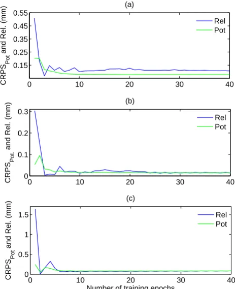
Figure 7 illustrates the evolution of both components of the CRPS with the number of training epochs. For Le Golo and Leaf, both the potential CRPS and the reliability component
0 10 20 30 40
0.15 0.25 0.35 0.45 0.55
CRPS
Pot
and Rel. (mm)
(a)
0 10 20 30 40
0 0.1 0.2 0.3
CRPS
Pot.
and Rel. (mm)
(b)
0 10 20 30 40
0 0.5 1 1.5
Number of training epochs
CRPS
Pot
and Rel. (mm)
(c)
Rel Pot
Rel Pot
[image:7.595.51.285.326.513.2]Rel Pot
Fig. 7. Evolution of the Reliability and Potential CRPS with the number of training epochs for (a) Le Golo (b) Serein, and (c) Leaf Rivers. 27
Fig. 7. Evolution of the Reliability and Potential CRPS with the
number of training epochs for (a) Le Golo (b) Serein, and (c) Leaf Rivers.
sharply decrease in the first steps of the training process. Then, the reliability components increases a little, indicat-ing that the ensemble becomes less reliable, before stabi-lizing for the remaining of the training. The Serein River shows a similar pattern for the reliability component, but the potential CRPS initialy increases for the first few train-ing epochs before decreastrain-ing. Generally speaktrain-ing, the po-tential CRPS decreases (i.e. improves) as the training of the networks evolves, which is consistent with the fact that the MLPs turn into more accurate models.
1 11 21 31 41 51 0
0.1 0.2
Epoch #1
1 11 21 31 41 51 0
0.1 0.2
Epoch #2
1 11 21 31 41 51 0
0.1 0.2
Epoch #3
1 11 21 31 41 51 0
0.1 0.2
Epoch #4
1 11 21 31 41 51 0
0.1 0.2
Epoch #5
1 11 21 31 41 51 0
0.1 0.2
Epoch #6
1 11 21 31 41 51 0
0.1 0.2
Epoch #7
1 11 21 31 41 51 0
0.1 0.2
Epoch #8
1 11 21 31 41 51 0
0.1 0.2
Epoch #9
1 11 21 31 41 51 0
0.1 0.2
Relative Frequency
Epoch #10
1 11 21 31 41 51 0
0.1 0.2
Rank Epoch #20
1 11 21 31 41 51 0
0.1 0.2
[image:8.595.49.285.62.366.2]Epoch #40
Fig. 8.Rank histograms for epochs 1 to 10, 20 and 40 for the Le Golo River.
28
Fig. 8. Rank histograms for epochs 1 to 10, 20 and 40 for the
Le Golo River.
solution. This leads to sharp but underdispersed distribu-tions, as revealed by an overabundant occurrence of obser-vations ranked first or last in the histograms above epoch 8.
Reliability diagrams, again for Le Golo basin and for epochs 1 to 10, 20, and 40, are drawn in Fig. 9. The y -axis is the average effective coverage of the intervals while the nominal coverage is indicated on the plots for the 0.2, 0,4, 0.6 and 0.8 intervals. Thex-axis is the effective width of the intervals. The best situation is when the nominal and effective coverage of the intervals are identical, with the ef-fective width as short as possible (good resolution). On one hand, diagrams for epochs 1 to 4 show effective interval cov-erage that is greater than the nominal covcov-erage for all confi-dence intervals, corroborating overdispersed NN ensembles. On the other hand, reliability diagrams for epochs 7 to 10 show the opposite. The most reliable diagrams are obtained at epoch 5 and 6, when effective and nominal coverages al-most coincide.
Clearly, this experiment shows that the reliability of confi-dence intervals, computed from an ensemble of individually trained MLPs, varies as their training progresses. While the accuracy of the forecast computed by averaging the networks forming the ensemble improves with the number of training epochs, the reliability of the confidence intervals may be op-timal after only a few training epochs: five to ten for this
0 5
0 0.2 0.4 0.6 0.8 1
Epoch #1
0 3 6 9
Epoch #2
0 2.5 5
Epoch #3
0 1 2
0 0.2 0.4 0.6 0.8
1 Epoch #4
0 0.5 1 1.5 2
Epoch #5
0 0.5 1
Epoch #6
0 0.5
0 0.2 0.4 0.6 0.8
1 Epoch #7
Mean effective probability of the intervals 0 0.25 0.5 Epoch #8
0 0.25 0.5
Epoch #9
0 0.2 0.4
0 0.2 0.4 0.6 0.8
1 Epoch #10
Mean effective width of the intervals
0 0.2 0.4
Epoch #20
0 0.2 0.4
[image:8.595.313.543.65.377.2]Epoch #40
Fig. 9.Reliability diagrams for epochs 1 to 10, 20 and 40 for the Le Golo River.
29
Fig. 9. Reliability diagrams for epochs 1 to 10, 20 and 40 for the
Le Golo River.
experiment. Because this study does not attempt to account for all possible sources of uncertainty (especially the ones linked to the choice of the model architecture), it is not real-istic to aim for perfectly reliable confidence intervals. How-ever, we suggest that the results of such an experiment could also be useful to conduct tests on various post-processing methods (e.g. Wilks and Hamill, 2007). All possible situa-tions for raw probabilistic or ensemble forecasts are repre-sented in the results: overdispersion at the beginning of the training, underdispersion at the end, presence of bias to dif-ferent extent, and some situations where the distribution is almost reliable.
5 Conclusions
epoch of the training process. We have assessed the reliabil-ity of those intervals and compared the performance of the ensembles with their average value, comparing the MAE and the CRPS. We have also applied the mean logarithmic score and showed that it evolves differently than the mean CRPS as training is performed. Finally, we have also broken the CRPS into its potential and reliability components and showed that its reliability component improves drastically within the first few training epochs: a characteristic that was corroborated by the reliability diagrams and by the rank histograms.
During this experiment, we noted that the CRPS was consistently lower than the MAE, regardless of the number of training epochs. This suggests that it is altogether more advantageous to work with the fifty issued forecasts than to use only their average value. However, because the MLP ensembles constructed here do not account for all possible sources of uncertainties in the streamflow forecasting situation, computed confidence intervals are not reliable, especially after the networks have been trained for more than 10 epochs. Nonetheless, considering the simplicity of implementation of an ensemble of MLPs, especially in contrast with a standard hydrological ensemble prediction system that relies on a complex rainfall-runoff model and on meteorological ensemble forecasts, catchment stakeholders and managers may consider this option as a first order mean to compute close to be reliable short-term streamflow forecasts.
Edited by: E. Toth
References
Abrahart, R. J. and See, L.: Comparing neural network and autore-gressive moving average technique for the prevision of continu-ous river flow forecasts in two contrasting catchments, Hydrol. Process., 14, 2157–2172, 2000.
Anctil, F., Filion, M., and Tournebize, J.: A neural network ex-periment on the simulation of daily nitrate-nitrogen and sus-pended sediment fluxes from a small agricultural catchment, Ecol. Model., 220, 879–887, 2009.
Baringhaus, L. and Franz, C.: On a new multivariate two-sample test, J. Multivariate Anal., 88, 190–206, 2004.
Ajami, N., Duan, Q., and Sorooshian, S.: An integrated hy-drologic Bayesian multimodel combination framework: Con-fronting input, parameter, and model structural uncertainty in hydrologic prediction, Water Resour. Res., 43, W01403, doi:10.1029/2005WR004745, 2007.
Anctil, F. and Lauzon, N.: Generalisation for neural networks through data sampling and training procedures, with applications to streamflow predictions, Hydrol. Earth Syst. Sci., 8, 940–958, 2004,
http://www.hydrol-earth-syst-sci.net/8/940/2004/.
Breiman, L.: Bagging predictor, Mach. Learn., 24, 123–140, 1996. Campolo, M., Andreussi, P., and Soldati, A.: River flood forecasting with neural network model, Water Resour. Res., 35, 1191–1197, 1999.
Carney, M., Cunningham, P., Dowling, J., and Lee, C.: Predict-ing probability distributions for surf height usPredict-ing an ensemble of mixture density networks, 22nd International Conference on Machine Learning, Bonn, Germany, 2005.
Coulibaly, P., Anctil, F., and Bobb´ee, B.: Hydrological forecasting with neural networks: The state of the art, Can. J. Civil Eng., 26, 293–304, 1999.
Crespo, J., Mora, E., and Peire, J.: Estimation Performance of Neu-ral Networks, 531–534, IEEE International Symposium on In-dustrial Electronics ISIE’93, Budapest, Hungary, 1993. Cybenko, G.: Approximation by superposition of a sigmoiddal
function, Math. Control Signal., 2, 303–314, 1989.
Efron, B. and Tibshirani, R.: An introduction to the bootstrap, edited by: Cox, D. R., Hinkley, D. V., and Reid, N., Hall, Lon-don, 1993.
Freitas, P. S. A. and Rodrigues, A. J. L.: Model combination in neural-based forecasting, Eur. J. Oper. Res., 173, 801–814, 2006. Freund, Y. and Shapire, R. E.: Experiments with a new boosting algorithm, in: Proc. of 13th International Conference on Machine Learning, edited by: Saitta, L., Bari, Italy, Morgan Kaufmann, San Francisco, CA, USA, 148–156, 1996.
Gneiting, T. and Raftery, A.: Strictly proper scoring rules, predic-tion, and estimapredic-tion, J. Am. Stat. Assoc., 102, 359–378, 2007. Good, I.-J.: Rational Decisions, J. Roy. Stat. Soc. B, 14, 107–114,
1952.
Hamill, T. and Colucci, S.: Verification of eta-RSM short-range en-semble forecasts, Mon. Weather Rev., 125, 1312–1327, 1997. Hansen, L.-K.-H. and Salamon, P.: Neural network ensembles,
IEEE T. Pattern Anal., 12, 993–1001, 1990.
Hersbach, H.: Decomposition of the continuous ranked probability score for ensemble prediction systems, Weather Forecast., 15, 550–570, 2000.
Hornik, K., Stinchcombe, M., and White, H.: Multilayer feedfor-ward networks are universal approximators, Neural Networks, 2, 359–366, 1989.
Hsieh, W.-W. and Tang, B.: Applying neural network models to prediction and data analysis in meteorology and oceanography, B. Am. Meteorol. Soc., 79, 1855–1870, 1998.
Iyer, M.-S and Rhinehart, R.-R: A method to determine the required number of neural-network training repetitions, IEEE T. Neural Networ., 10, 427–432, 1999.
Jolliffe, I. and Stephenson, D.: Forecast Verification: A Practi-tioner’s Guide in Atmospheric Sciences, John Wiley and Sons, Chichester, 2003.
Kang, K.-W., Park, C.-Y., and Kim, J.-H.: Neural network and its application to rainfall-runoff forecasting, Korean J. Hydrosci., 4, 1–9, 1993.
Karunanithi, N., Grenney, W.-J., Whitley, D., and Bovee, K.: Neural networks for river flow prediction, J. Comput. Civil Eng., 8, 201– 220, 1994.
Khan, M. and Coulibaly, P.: Bayesian neural network for rainfall-runoff modeling, Water Resour. Res., 42, W07409, doi:10.1029/2005WR003971, 2006.
Klemeˇs, V.: Operational testing of hydrological simulation models, Hydrolog. Sci. J., 31(1), 13–24, 1986.
Knutti, R., Stocker, T.-F., Joos, F., and Plattner, G.-K.: Probabilis-tic climate change projections using neural networks, Clim. Dy-nam., 21, 257–272, 2003.
Kohonen, T.: The Self-organizing map, Proc. IEEE, 79, 1464–1480, 1990.
Lajbcygier, P.-R. and Connor, J.-T.: Improved option pricing us-ing articial neural networks and bootstrap methods, Int. J. Neural Sys., 8, 457–471, 1997.
Levenberg, K.: A Method for the solution of certain non-linear problems in least squares, Q. Appl. Math., 2, 164–168, 1944. Mackay, D.: A pratctical Bayesian framework for backpropagation
networks, Neural Comput., 4, 448–472, 1992.
Maier, H.-R. and Dandy, G.-C.: Neural Networks for the prediction and forecasting of water resources variables: A review of mod-eling issues and applications, Environ. Modell. and Softw., 15, 101–124, 2000.
Marquardt, D.: An algorithm for least-squares estimation of nonlin-ear parameters, SIAM J. Appl. Math., 11, 431–441, 1963. Neal, R.: Bayesian learning for neural networks, Springer, New
York, 1996.
Papadopoulos, G. and Edwards, P.-J.: Confidence estimation meth-ods for neural networks: A practical comparison, IEEE T. Neural Network., 12, 1278–1287, 2001.
Rosenblatt, F.: The perceptron: A probabilistic model for infor-mation storage and organization in the brain, Psychol. Rev., 65, 386–408, 1958.
Roulston, M.-S. and Smith, L.-A.: Evaluating probabilistic fore-casts using information theory, Mon. Weather Rev., 130, 1653– 1660, 2002.
Shrestha, D.-L. and Solomatine, D.-P.: Experiments with Asa-Boost.RT, an improved boosting scheme for regression, Neural Comput., 18(7), 1678–1710, 2006.
Shrestha, D.-L. and Solomatine, D.-P.: Machine learning ap-proaches for estimation of prediction interval for the model out-put, Neural Networks, 19, 225–235, 2006.
Singh, P. and Deo, M.: Suitability of different neural networks in daily flow forecasting, Appl. Soft Comput., 7, 968–978, 2007. Sz´ekely, G.J. and Rizzo, M.L.: A New Test for Multivariate
Nor-mality, J. Multivariate Anal., 93, 58–80, 2005.
Talagrand, O., Vautard, R., and Strauss, B.: Evaluation of proba-bilistic prediction systems., ECMWF Workshop on Predictabil-ity, Shinfield Park, Reading, Berkshire, 1–25, 1997.
Tokar, A.-S. and Johnson, P.-A.: Rainfall-runoff modeling using ar-tificial neural networks, J. Hydrol. Eng., 4, 232–239, 1999. Valverde Ram´ırez, M.-C., De Campos Velho, H.-F., and
Fer-reira, N.-J.: Artificial neural network technique for rainfall fore-casting applied to the S˜ao Paulo region, J. Hydrol., 301(1–4), 146–162, 2005.
Vel´azquez, J. A., Petit, T., Lavoie, A., Boucher, M.-A., Turcotte, R., Fortin, V., and Anctil, F.: An evaluation of the Canadian global meteorological ensemble prediction system for short-term hy-drological forecasting, Hydrol. Earth Syst. Sci., 13, 2221–2231, 2009,
http://www.hydrol-earth-syst-sci.net/13/2221/2009/.
Wilks, D. and Hamill, T.: Comparison of ensemble-MOS meth-ods using GFS reforecasts, Mon. Weather Rev., 135, 2379–2390, 2007.
Wilks, D.-S.: Statistical Methods in the Atmospheric Sciences, Academic Press, San Diego, 1995.