Linking Financial Development and Total Factor Productivity of the Philippines

(1)

Munich Personal RePEc Archive

Linking Financial Development and Total

Factor Productivity of the Philippines

Calub, Renz Adrian

University of the Philippines School of Economics (UPSE)

March 2011

Online at

https://mpra.ub.uni-muenchen.de/66042/

(2)

1 Linking Financial Development and Total Factor Productivity of the

Philippines

*

Renz Adrian T. Calub

**

Abstract: Financial development is said to have an impact on growth. In this paper we try to extend this notion to total factor productivity. As Bianchi [2010] noted, easing access to capital may encourage entrepreneurship and thus productivity. To test this relationship, we use

Cororaton and Cuenca’s [2001] estimates of TFP and World Bank’s M3 to GDP (liquid liabilities

to GDP) as a measure of financial depth. Estimates from our vector error correction model suggest that there is indeed a dynamic relationship between financial development and TFP.

Keywords: Financial development, total factor productivity, VECM JEL: G2, O4

*_{This paper serves as a partial fulfillment of the requirements for Macroeconomic Theory. Date Submitted: March}

2011

**_{MA Economics, University of the Philippines School of Economics, Diliman, Quezon City 1101. Email:}

(3)

2

Introduction

Theory suggests a strong relationship between financial development and economic growth. Financial development is defined by Levine and Demirguc-Kunt [2008] as the reduction, if not elimination, of information, enforcement, and transaction costs faced by financial intermediaries in mobilizing capital, managing risk, optimizing investment allocation, and lubricating trade of goods. Economists such as Schumpeter [1911] and Gurley and Shaw [1955] claim that financial intermediaries can efficiently channel funds to more productive economic agents (i.e. firms), which implies higher output and incentives to improve technology. Furthermore, with the

financial intermediaries’ information advantage, lenders are encouraged to lend without worrying about the safety of their savings.

Cross-country empirical evidences support these propositions. King and Levine [1993], Goldsmith [1969], McKinnon [1973] and several regional studies present evidence of links between financial development and economic growth. These studies, however, gauged growth in terms of Gross Domestic Product (GDP). While widely used for growth, GDP may be too broad a measure. Financial development implies ease, if not increase, in capital formation and along with this capital formation are knowledge spillovers which increase productivity. As Cypher and Dietz [2008] discussed, GDP measures extensive economic growth arising from higher levels of input. On the other hand, TFP measures intensive economic growth, the

“synergistic effect of combining an economy’s physical and its human capital” [p. 431]. Therefore, TFP may be a more effective measure in assessing the influence of financial development to productivity as theorists have claimed.

In this light, we shall assess the relationship between financial development and TFP in the Philippines. Using basic time series modeling techniques we shall test whether there is a long-run relationship between financial development and TFP. Further, we shall also describe their short run dynamics and find out whether they converge towards a stable equilibrium.

This paper shall be divided into 4 sections. First we revisit the literature on financial development and growth. Section 2 presents the methodology where we discuss the indices for financial development and total factor productivity. Section 3 presents the results and some discussion. Section 4 concludes.

Literature Review

Schumpeter in 1911 may have been the first to point out the power of the financial intermediaries. Its ability to channel funds from frugal consumers to innovative firms can spell technological innovation and economic growth. As an institution holding savings for consumers, they (ought to) have the information advantage regarding riskiness and profitability of investments [Levine and King 1993].

(4)

3

Much like Schumpeter, Gurley and Shaw1_{noted that economic development involves finance.}

Decisions on spending, saving, investment, income and wealth generation, in their terms, revolve around the financial sector.

Pagano [1993] formulated a mathematical support for these arguments. He provided the analytical foundation for the empirical papers relating financial development to growth. With a simple endogenous model, he came up with a steady-state growth rate equation that includes financial development.

𝑔 = 𝐴𝜑𝑠 − 𝛿 (1)

Where 𝑔 is the steady-state growth rate, 𝐴 is the social marginal productivity for capital, 𝜑 is the fraction of savings that goes to investment, and 𝑠 is the private savings rate. Pagano explains that financial intermediation influences growth through these three channels: 𝐴, 𝑠, and 𝜑. Precisely, the development of the financial sector can prop up 𝜑, the proportion of savings that go to investment,2_increase_𝐴_{by placing funds over projects with higher marginal product of}

capital, and encourage savings 𝑠.3

While these theories sound plausible, there are some economists who dismiss this relationship. Joan Robinson [1952] argued that it is the development of the real economy that drives the development of the financial sector. Rather than the financial sector creates incentives for firms to innovate, it is these firms who initiate creativity and push the financial intermediaries to develop. Interestingly, if Gurley and Shaw [1955] lamented the lack of attention given to financial intermediaries, Robert Lucas [1988: 6] cried “overstress” to the financial sector.

These propositions focused primarily on aggregate income as a growth measure. In the following sections we visit existing literature on financial depth and total factor productivity.

On financial development and productivity in the form of entrerpreneurship

Bianchi [2010] proposed the interaction between labor markets, financial markets, and production technologies. In this theoretical paper, he first established the importance of financial institutions in encouraging entrepreneurship. Individuals, depending on their circumstances, may choose to be self-employed, employed in a firm, or set up their own business. Easing credit allows talented entrepreneurs to build their own firms, increasing productivity and competition while at the same time discouraging less talented individuals to compete. As more talented entrepreneurs set up their own firms, less productive firms and technologies are driven out of the economy, thus increasing productivity.

That is one side of the story. There are, however, impediments on financial development driven mainly by individual incentives in the labor market. Arising from the lack of sufficient information on entrepreneurial talent, banks are unable to gauge an individual’s ability to run a firm, add to that the possibility that the debtor may not even use the capital to productive investments. With this information asymmetry, banks are forced to implement collaterals.

1_{In this paper, Gurley and Shaw [1955] seemed to lament the lack of attention given to finance by other economists.} 2_{The remaining}_{(1 − 𝜑)}_{goes to the banking sector in the form of interest rate spreads or costs. This implies that}

inefficient financial intermediaries may have higher (1 − 𝜑), and thus lower 𝜑 which should have been used for investment.

3_{Pagano, however, came up with ambiguous results on the savings rate effect, noting that the ease of access to}

(5)

4

He further states that the tight credit flow comes from the interaction of the labor market and financial markets. If there are few entrepreneurs, then labor demand is low and given the circumstances, the unemployed have no choice but to try borrowing. Because of this, banks may have to set up high collaterals to screen bad debtors; hence, entrepreneurship is further dampened. On the positive note, high entrepreneurship implies higher labor demand. Low unemployment means that those who demand for loans are more likely to be credit worthy and highly-skilled entrepreneurs. This in turn reduces the need for higher collateral levels and thus encourages more entrepreneurship.

Empirical evidence

Theories posit that financial development props up growth through encouraging innovations and productivity, and empirical literature supports this stance. Arizala, Cavallo, and Galindo [2009] used a panel of 77 countries from 1963 to 2003 and measured industry-level total factor productivity against financial dependence of the industry interacted with a proxy for financial development. Results show that the effect of financial development in improving productivity hinges on the volatility of the macroeconomy, particularly with regards to inflation. While financial development drives TFP as volatility increases, too much of it dampens this effect.

Guiso, Sapienza, and Zingales [2004] conducted a single-country study on Italy. They developed a measure of local financial development reflecting the theory of Gurley and Shaw [1955]. Results show that amid the financial integration across Italy, local financial institutions still do matter as they encourage entrepreneurship, attract other firms, and thus improve growth. Furthermore, results show differences in the effect of financial development between large and small firms.

Aside from directly influencing the total factor productivity, one empirical study showed evidence that financial development also channels the effect of foreign direct investments towards TFP. Alfaro, Kalemli-Ozcan, and Sayek [2009] presented this using simple OLS on 62 countries within the period 1975-1995.4_{Results show that FDI benefits are not all about factor}

accumulation. Evidence shows that financial development aids the translation of FDI to improvements in TFP.

Since financial development moves alongside aggregate output, it should follow that improving financial sectors and easing capital flows must also improve productivity, as captured by the 𝐴

variable in Pagano’s model. Similarly, financial development may even allow for reduction of

information asymmetry and thus invoke the positive effects to entrepreneurship proposed by Bianchi [2010]. Effectively, TFP is a broader measure of capital since it accounts for intangible capital (i.e. human knowledge) [Prescott 1998] and as predicted by the neoclassical Solow growth model, capital is an essential factor to growth.

Methodology

Before proceeding to the actual estimation, we will first come up with total factor productivity estimates whose procedures were formulated by Cororaton and Cuenca [2001]. Assuming a

4_{Their study also measured the relationship between economic growth, financial development, and FDI for a sample}

(6)

5

neo-classical production function, price-taking and maximizing behavior, TFP is estimated using a translog model:

𝑇𝐹𝑃𝑡 = ∆ ln 𝑄𝑡− 𝑎𝑁∆ ln 𝑁𝑡− 𝑎𝐾∆ ln 𝐾𝑡 ₍₂₎

𝑄𝑡 is the annual output. 𝑁𝑡 and 𝐾𝑡 are labor and capital in log form and differentiated by one

year. Meanwhile, 𝑎_𝑁 and 𝑎_𝐾 are average factor shares. This formula is a modification of the Solow Residual using Tornqvist index for discrete data [Cororaton and Cuenca 2001].5

We will explicitly use one of the financial development indicators formulated by King and Levine [1993]. After estimating total factor productivity, we proceed to estimating its relationship with financial development, as denoted by the basic VAR model:

𝒀𝑡 = 𝜸 + 𝐴1𝒚𝑡−1+ 𝐴𝟐𝒚𝒕−𝟐+ ⋯ + 𝐴𝑝𝒚𝑡−𝑝+ 𝒗𝑡 (3)

Where 𝒀_𝑡 is a 𝑀 × 1 vector containing TFP and the financial development indicators, 𝜸 is the vector of means, 𝐴_𝑝 are the 𝑀 × 𝑀 matrix of parameters, and 𝒗_𝑡 is a random term [Greene 1997]. This VAR model shall be the benchmark model to test the relationship between financial development and economic growth. This setup allows us to use Granger Causality to assess whether past financial market innovations influence total factor productivity or possibly the other way around [Wooldridge 2006].6_{VAR models, or Vector Error Correction models in the}

restricted sense, has been used by several studies dealing with financial development indicators and growth, as can be seen in studies cited in Walsh [2000]7_.

Unrestricted vector autoregression, however, cannot be undertaken especially when dealing with macroeconomic variables. Inherent characteristics of these time series variables, such as integrated processes, may lead to spurious regression if OLS estimation is used right ahead [Wooldridge 2006]. Therefore, the variables shall undergo several tests widely used in dealing with time-indexed macroeconomic variables.

Stationarity

Variables that exhibit changing mean and variance across time are said to be non-stationary and may pose problems in inference [Wooldridge 2006]. Formally, highly persistent time series can be denoted by AR(1) models whose parameter is equal to one. One example is the random walk.8_{To address this, Dickey and Fuller (1979, 1981) developed a test to identify persistence}

in a series. Consider the following AR(𝑝 − 1) model [Greene 1997]:

∆𝑦𝑡 = 𝛿 + 𝜌𝑦𝑡−1+ ∑ 𝜑𝑗 𝑝−1

𝑗=1

∆𝑦𝑡−𝑗+ 𝜀𝑡 (4)

5_{We will explicitly follow the TFP estimation procedures of the said paper. Given the limitations of data sources,}

some of the variables, particularly capital stock, shall also be estimated.

6_{See Greene [1997] and Wooldridge [2006] for a comprehensive treatment on VAR models and Granger Causality.} 7_{Studies involve measuring long-run effects of money to growth.}

8_{Econometrics textbooks such as that of Greene [1997] and Wooldridge [2006] have a comprehensive discussion on}

(7)

6

From this equation, we test the null hypothesis that 𝜌 = 0. Failure in rejecting the null hypothesis is sufficient to say that no unit root exists in the variable’s first-differenced form. This procedure can easily be done by statistical software.

Cointegration

Integrated of order 1 or I(1) variables, while cannot be regressed explicitly, has some implications on long-run relationships. As presented by Engle and Granger [1987], variables are cointegrated of order 1 if their linear combinations are stationary. Formally a vector of I(1) variables 𝑥_𝑡 are said to be cointegrated if:

𝑧𝑡 = 𝜑′𝑥𝑡 ~ I(0) (5)

Where 𝜑′ is called the cointegrating vector. This can also be extended to multivariable case, where (3) will be in matrix form instead of vectors. Cointegration suggests that the vector of variables do not deviate from an equilibrium level 𝑧_𝑡 that is dynamically stable, invoking a long-run relationship between them [Engle and Granger 1987].

Testing for cointegration, in the theoretical sense, means testing for significance of the cointegrating vector 𝜑. While the actual procedures for testing are quite complicated and critical values are difficult to derive [Wooldridge 2006], this can easily be done by statistical software.

Error-correction model

Engle [1983] postulated the representation of cointegrating variables using error correction terms with his formulation of Granger Representation Theorem. Even with the existence of cointegrating variables, we still have a way to use VAR models by including an error-correction term to capture the cointegration [Engle and Granger 1987]. This modifies Equation 3:

∆𝒀𝑡 = 𝜸 + 𝐴1∆𝒚𝑡−1+ ⋯ + 𝐴𝑝∆𝒚𝑡−𝑝+ 𝜹𝒌′𝒛𝑘+ 𝒗𝑡 ₍₆₎

Where 𝒛_𝑘 is the vector of cointegrating variables as we defined in Equation 5. Note that this setup allows us not only to determine the existence of long-run relationship between financial development and TFP but also the short-dynamics or how the variables tend towards the equilibrium [Wooldridge 2006].

Data and Results

Considering the data limitations, we shall explicitly utilize the estimates of Cororaton and Cuenca [2001] of TFP, depreciation, and capital stock series from 1980-1999. From there, we estimate the TFP for the succeeding years using data from International Labor Organization, National Statistical Coordination Board (NSCB), and IDEA Inc. (see Appendix A for the data table). Meanwhile, since we are limited to annual series (i.e. 1981-2008) we shall use only The

World Bank’s ratio of liquid liabilities (M3) to GDP data as used by King and Levine [1993].9_As

such, our VAR or VECM model reduces to two-variable case.

9_{King and Levine [1993] noted that the ratio of liquid liabilities to GDP is a traditional measure of financial depth.}

(8)

7

Results

Test for stationarity suggests the existence of unit root test at levels. The nonstationarity problem, nevertheless, is eliminated with first differencing. We present it in the following table:

Notice that the two variables are stationary at 5 percent level of significance for models with intercept and trend. The number of lags is specified according to Schwartz Information Criterion, which is automatically determined using the statistical software.

Given that the variables are I(1), we test for cointegration to know whether we need to restrict our VAR model to VECM. The following table shows the results:

Assuming that there is no deterministic trend in the variables, there is at least 1 cointegrating equation at 5 percent level of significance (see p-values). The lags used were again derived from Schwartz Information Criterion. This leads us to account for a vector error correction term in our VAR model.

Table 1. Augmented Dickey-Fuller Test

[image:8.612.141.499.600.721.2]

Table 2. Johansen Cointegration Test

(9)

8

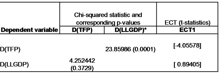
The Vector Error Correction model yields some interesting results as shown in the Table 3. The Granger Causality test shows that the lagged differences of LLGDP (our indicator for financial development) granger-cause TFP. Furthermore, the significance of the error-correction term verifies the long-run relationship we already know from the cointegration test. Notice that the negative error-correction term implies that when LLGDP deviates much from TFP, productivity catches up, since 𝒛_𝑡 becomes negative. Similarly, when productivity deviates from equilibrium, the error-correction parameter “corrects” it [Wooldridge 2006]. On the other hand, total factor productivity does not granger-cause financial development. The error-correction term is also not statistically significant.

With our vector error correction model we have empirically shown that financial development is dynamically correlated with productivity in the long run. As theory has shown, ease of credit may encourage entrepreneurship and thus contribute to productivity.

Since total factor productivity may not be tangible as physical capital (i.e. education), banks may still be reluctant to provide credit. Although people have the sufficient education or technical know-how to set up a firm, amid the adverse selection problems [Bianchi 2010], banks may not still be willing to lend capital. Hence the granger-non-causality of TFP to financial development; banks ex ante cannot identify whether borrowers have sufficient productivity and know-how so they are reluctant to lend financial capital.

Conclusions and Recommendations

In this paper we have shown the relationship between financial development and total factor productivity. Starting with theories that relate financial depth to GDP, we extended this to the concept of productivity, arguing that easing capital flows through financial institutions may encourage entrepreneurship and hence productivity. Using TFP data from Cororaton and Cuenca [2001] and M3 to GDP ratio from World Bank, we estimated the dynamic relationship between total factor productivity and financial development. Results are consistent with the theories presented: financial development encourages productivity.

(10)

9

References:

Alfaro, Laura; Kalemli-Ozcan, S.; Sayek S. (2009) “FDI, Productivity, and Financial

Development”. World Economy 32 (1), 111-135

Arizala, Francisco, Cavallo, E., & Galindo, A., (2009, Jun). Financial Development and TFP Growth: Cross-Country and Industry-Level Evidence. Inter-American Development Bank Working Paper #682. Retrieved 20 Jan 2010, from www.iadb.org/research/pub_hits.cfm? pub_id=2036022.

Bianchi, Milo (2010). “Credit Constraints, entrepreneurial talent, and economic development”.

Small Business Economics 34: 93-104

Cororaton, C., & Cuenca, J., (2001). Estimates of Total Factor Productivity in the Philippines. PIDS Discussion Paper Series # 2001-02. Retrieved 1 Dec 2010 from dirp4.pids.gov.ph/ris/pdf/ pidsdps0102.pdf.

Cypher, James and Dietz, James L. (2008). The Process of Economic Development. Taylor and Francis Group.

Engle, Robert and Granger, C.W.J. (Mar 1987). “Co-Integration and Error Correction: Representation, Estimation, and Testing,”Econometrica 55 (2), 251-276.

Greene, William J. (1997) Econometric Analysis. New Jersey: Prentice Hall.

Guiso, L., Sapienza, P., & Zingales, L. (2004). “Does Local Financial Development Matter?”,

The Quarterly Journal of Economics 119 (3), 929-969.

Gurley, John, and Shaw, E.S. (1955). “Financial Aspects of Economic Development,”The American Economic Review 45 (4). 515-538

King, R. G., & Levine, R. (1993). Finance and Growth: Schumpeter Might Be Right. Washington D.C.: The World Bank Policy Research Department.

Pagano, M. (1993). “Financial Markets and Growth: An Overview,” European Economic Review 37 , 613-622.

Robinson, J. (1952). "The Generalization of the General Theory". In The Rate of Interest and Other Essays. London: MacMillan.

Schumpeter, J. (1911). The Theory of Economic Development. Cambridge: Harvard University Press.

(11)

10

Appendix – Estimation results

Null Hypothesis: D(TFP) has a unit root Exogenous: Constant

Lag Length: 2 (Automatic based on SIC, MAXLAG=6)

t-Statistic Prob.*

Augmented Dickey-Fuller test statistic -3.380653 0.0221 Test critical values: 1% level -3.737853

5% level -2.991878 10% level -2.635542

*MacKinnon (1996) one-sided p-values.

Augmented Dickey-Fuller Test Equation Dependent Variable: D(TFP,2)

Method: Least Squares Date: 02/19/11 Time: 22:44 Sample (adjusted): 1985 2008

Included observations: 24 after adjustments

Variable

Coefficie

nt Std. Error t-Statistic Prob.

D(TFP(-1))

-1.098901 0.325056 -3.380653 0.0030 D(TFP(-1),2) 0.157430 0.290365 0.542179 0.5937 D(TFP(-2),2) 0.435780 0.199910 2.179882 0.0414 C 0.003723 0.004376 0.850713 0.4050

R-squared 0.714566 Mean dependent var

-0.000944 Adjusted R-squared 0.671751 S.D. dependent var 0.036181

S.E. of regression 0.020729 Akaike info criterion

-4.763529

Sum squared resid 0.008594 Schwarz criterion

(12)

11

Null Hypothesis: D(TFP) has a unit root Exogenous: Constant, Linear Trend

t-Statistic Prob.*

5% level -3.612199 10% level -3.243079

Variable

Coefficie

D(TFP(-1))

-1.098484 0.332823 -3.300504 0.0038 D(TFP(-1),2) 0.162428 0.297840 0.545353 0.5919 D(TFP(-2),2) 0.441060 0.205558 2.145670 0.0450 C 0.000999 0.010744 0.092955 0.9269 @TREND(1981) 0.000176 0.000630 0.278925 0.7833

-4.684282

(13)

12

Null Hypothesis: D(TFP) has a unit root Exogenous: Constant, Linear Trend

t-Statistic Prob.*

5% level -3.612199 10% level -3.243079

Variable

Coefficie

D(TFP(-1))

-1.098484 0.332823 -3.300504 0.0038 D(TFP(-1),2) 0.162428 0.297840 0.545353 0.5919 D(TFP(-2),2) 0.441060 0.205558 2.145670 0.0450 C 0.000999 0.010744 0.092955 0.9269 @TREND(1981) 0.000176 0.000630 0.278925 0.7833

-4.684282

(14)

13

Null Hypothesis: D(LLGDP) has a unit root Exogenous: Constant

t-Statistic Prob.*

5% level -2.991878 10% level -2.635542

Augmented Dickey-Fuller Test Equation Dependent Variable: D(LLGDP,2) Method: Least Squares

Date: 02/19/11 Time: 22:45 Sample (adjusted): 1984 2007

Variable

Coefficie

D(LLGDP(-1))

-0.609475 0.267400 -2.279260 0.0332

D(LLGDP(-1),2)

-0.391580 0.198114 -1.976541 0.0614 C 0.004582 0.007668 0.597513 0.5566

-3.811462

(15)

14

Null Hypothesis: D(LLGDP) has a unit root Exogenous: Constant, Linear Trend

t-Statistic Prob.*

5% level -3.603202 10% level -3.238054

Variable

Coefficie

D(LLGDP(-1))

-0.992368 0.216001 -4.594280 0.0001 C 0.022880 0.017014 1.344797 0.1924

@TREND(1981)

-0.000820 0.001052 -0.779979 0.4437

-3.603450

(16)

15

Null Hypothesis: D(LLGDP) has a unit root Exogenous: None

t-Statistic Prob.*

5% level -1.955681 10% level -1.608793

Variable

Coefficie

D(LLGDP(-1))

-0.541204 0.238201 -2.272045 0.0332

D(LLGDP(-1),2)

-0.424079 0.187697 -2.259387 0.0341

-3.877937

(17)

16

Included observations: 22 after adjustments Trend assumption: No deterministic trend Series: TFP LLGDP

Lags interval (in first differences): 1 to 4

Unrestricted Cointegration Rank Test (Trace)

Hypothesized Trace 0.05

No. of CE(s) Eigenvalue Statistic Critical Value Prob.**

None * 0.543927 17.41694 12.32090 0.0064 At most 1 0.006556 0.144706 4.129906 0.7535

Trace test indicates 1 cointegrating eqn(s) at the 0.05 level * denotes rejection of the hypothesis at the 0.05 level **MacKinnon-Haug-Michelis (1999) p-values

Unrestricted Cointegration Rank Test (Maximum Eigenvalue)

Hypothesized Max-Eigen 0.05

No. of CE(s) Eigenvalue Statistic Critical Value Prob.**

None * 0.543927 17.27224 11.22480 0.0039 At most 1 0.006556 0.144706 4.129906 0.7535

Max-eigenvalue test indicates 1 cointegrating eqn(s) at the 0.05 level * denotes rejection of the hypothesis at the 0.05 level

**MacKinnon-Haug-Michelis (1999) p-values

Unrestricted Cointegrating Coefficients (normalized by b'*S11*b=I):

TFP LLGDP -92.36340 5.382875 9.183228 3.752923

Unrestricted Adjustment Coefficients (alpha):

D(TFP) 0.010737 -2.17E-06 D(LLGDP) -0.000950 0.001927

1 Cointegrating Equation(s): Log likelihood 121.4990

(18)

17

TFP LLGDP 1.000000 -0.058279

(0.01173)

Adjustment coefficients (standard error in parentheses) D(TFP) -0.991734

(19)

18

Vector Error Correction Estimates Date: 02/19/11 Time: 22:47 Sample (adjusted): 1986 2007

Included observations: 22 after adjustments Standard errors in ( ) & t-statistics in [ ]

Cointegrating Eq: CointEq1

TFP(-1) 1.000000

LLGDP(-1) -0.094121 (0.02216) [-4.24744]

C 0.029116

Error Correction: D(TFP) D(LLGDP)

CointEq1 -1.000171 0.511394 (0.24660) (0.57200) [-4.05578] [ 0.89405]

D(TFP(-1)) 0.315775 -0.383274 (0.20680) (0.47968) [ 1.52693] [-0.79902]

D(TFP(-2)) 0.407630 -0.566985 (0.13608) (0.31563) [ 2.99559] [-1.79636]

D(TFP(-3)) -0.185651 -0.012999 (0.18174) (0.42153) [-1.02154] [-0.03084]

D(TFP(-4)) 0.321008 -0.439650 (0.27077) (0.62805) [ 1.18554] [-0.70003]

D(LLGDP(-1)) -0.278076 0.208292 (0.12990) (0.30131) [-2.14062] [ 0.69128]

(20)

19

D(LLGDP(-3)) -0.448660 0.225000 (0.13947) (0.32349) [-3.21696] [ 0.69553]

D(LLGDP(-4)) -0.099921 0.089948 (0.14834) (0.34407) [-0.67360] [ 0.26142]

C 0.011516 0.009179 (0.00607) (0.01408) [ 1.89767] [ 0.65207]

R-squared 0.835700 0.491602 Adj. R-squared 0.712476 0.110303 Sum sq. resids 0.001966 0.010578 S.E. equation 0.012800 0.029690 F-statistic 6.781922 1.289284 Log likelihood 71.33351 52.82386 Akaike AIC -5.575774 -3.893078 Schwarz SC -5.079846 -3.397150 Mean dependent 0.001797 0.012822 S.D. dependent 0.023871 0.031476

Determinant resid covariance (dof

adj.) 1.39E-07

(21)

20

VEC Granger Causality/Block Exogeneity Wald Tests Date: 02/19/11 Time: 22:48

Sample: 1981 2008 Included observations: 22

Dependent variable: D(TFP)

Excluded Chi-sq df Prob.

D(LLGDP) 23.85986 4 0.0001

All 23.85986 4 0.0001

Dependent variable: D(LLGDP)

Excluded Chi-sq df Prob.

D(TFP) 4.252442 4 0.3729