Implementation of technological breakthroughs at sector level and the technology bias

Implementation of technological

breakthroughs at sector level and the

technology-bias

Stijepic, Denis and Wagner, Helmut

FernUniversität in Hagen

22 February 2011

Online at

https://mpra.ub.uni-muenchen.de/33352/

Implementation of technological breakthroughs at sector level and

the technology-bias

by

Denis Stijepic

University of Hagen, Germany

and

Helmut Wagner

University of Hagen, Germany

Contact Details:

Department of Economics

University of Hagen

Universitaetsstrasse 41

D-58084 Hagen

GERMANY

Tel: +49 2331 987 2640

Fax:+49 2331 987 391

e-mail: [email protected]

or: [email protected]

September 2011

Abstract

Different goods are produced by different sectors in an economy. The fact that sectors use different production technologies is named technology-bias. The technology-bias is well documented and has important theoretical implications for economic growth and unemployment. We provide a theoretical model that explains the technology-bias and its development. We provide empirical evidence on the development of the technology-bias and explain this development by using our model-results. Last not least, we discuss the implications of our findings for the existing growth literature and structural change literature.

Keywords: sector technology, implementation of technological progress, structural change, growth, multi-sector growth models

JEL-Codes: O14, O41

1

1. Introduction

Different goods are produced by different sectors in an economy. In general, we can say that

each sector has its own specific production technology. That is, technology differs across

sectors. This fact is named “cross-sector technology bias”. Many multi-sector models assume

the existence of such a technology bias and many models imply that this bias has important

impacts on the aggregate growth rate of the economy and on unemployment. (For some

references, see section 8.)

The aim of the paper is to provide a long-run growth model, which can explain the existence

of technology-bias endogenously. Especially, we focus on cross-sector bias regarding

capital-intensities, output-elasticities of capital and factor-income-shares. That is, we analyze why

output-elasticities of capital and thus capital-intensities differ across sectors and we analyze

how these differences develop over time. We also provide empirical evidence on this

question.

Our model is a sort of multi-sector Ramsey-Cass-Koopmans-model. General technology

breakthroughs are exogenous. They have to be implemented to improve the technology of

sectors. Implementation requires some creative ideas and, hence, depends upon the amount of

labor employed in a sector.

To our knowledge, the following literature is related to our paper:

1.) There is some literature, which endogenizes the cross-sector bias in TFP, for example

Acemoglu and Guerrieri (2006) and Ngai and Samaniego (2011). For an overview of this

literature, see Ngai and Samaniego (2011). In contrast to this literature, we focus on

endogenizing the cross-sector bias in output-elasticity of capital.2

2.) Zuleta and Young (2007) present a two-sector model where a “backward sector” uses

labor only and a “progressive sector” uses labor and capital; the output elasticity of capital in

the progressive sector can be increased by investment. Due to these assumptions the backward

sector cannot catch-up (since it cannot use capital), i.e. the technologies cannot converge. In

contrast, we focus on the catching-up process of the backward sector.

2

To see what the exact difference between our paper and the papers, which endogenize the TFP-growth rate, consider the paper by Acemoglu and Guerrieri (2006) as an example: The implicit sectoral production functions of Acemoglu and Guerrieri’s (2006)-model are depicted on page 15 of their paper (equation (27)). In fact these functions are of type Cobb-Douglas, like in our model. Acemoglu and Guerrieri (2006) endogenize the TFP ( and ) of these production functions on page 36 of their paper (equations (61)). Hence, we can say that the bias of TFP is endogenous in their model. However, the output-elasticities of inputs (

1

M M2

1

Our theoretical results imply that sectoral technologies may converge or diverge, depending

upon the sort of technological implementation (labor-augmenting or capital-augmenting),

structural change patterns (i.e. changes in factor-allocation across sectors), distribution of

capital-production across sectors and the nature of the breakthrough. Our empirical results

imply that sector-technologies converged between 1948 and 1987 in the USA, which may be

explained by prevalence of capital-augmenting technological implementation in the past

and/or increasing employment-shares of technologically backward sectors.

Overall, our model implies that models, which assume exogenous technology-bias, omit

important dynamics of structural change and aggregate growth. The reason is that

technology-bias tends to be self-reinforcing, causes structural change (cross-technology

factor-reallocation) and is affected itself by cross-technology factor reallocation. For a detailed

discussion of model-implications for the existing literature see section 8.

In the next section, we present the assumptions and the equilibrium of the model. In section 3

we discuss the dynamics of the model when no technological breakthroughs occur. In section

4 we study the impacts of a sequence of technology breakthroughs on the sectoral

technology-bias (via implementation). In section 5 we study how general structural-change-patterns affect

the implementation of breakthroughs at sector level. Section 6 provides a summary of the

factors which have an impact on the development of the technology-bias in our model. In

section 7 we provide some evidence on the development of the sectoral technology bias. In

section 8 we discuss the implications of our results for the existing literature. In section 9 we

provide some concluding remarks.

2 Model assumptions

2.1 Production

Assumption 1: Many heterogeneous goods (i=1,...n) are produced in the economy; each

good i is produced by a subsector i.

Assumption 2: Goods/subsectors i=1,...m are assigned to sector A; goods/subsectors

n m

i= +1,... are assigned to sector B ( . This is only a simplifying

assumption; in fact, our arguments work even when there are more than two

sectors.

)

m

n>

Assumption 3: Capital (K) and labor (L) are inputs in Cobb-Douglas production functions.

Assumption 4:Technology is homogenous within a sector but differs across sectors; i.e. there

is technology bias across sectors but not within sectors. For example, all

not the same technology as subsectors i=m+1,...n. Again, this is only a

simplifying assumption without implications for our main results. It helps us to

model the independency assumption in the next subsection.

Assumption 5: The degree of implementation of a general technological breakthrough

depends upon the number of persons who are employed in a sector. That is, the

more persons are employed in a sector, the better a technological breakthrough

is implemented. This is a very important assumption; it is discussed extensively

in Section 2.4.

Assumption 6: The implementation of a general technological breakthrough affects the

TFP-growth rate and the output elasticity of capital and labor respectively. That is,

implementation affects the marginal rate of technical substitution between

capital and labor and thus the optimal capital intensity of a sector. Again, this is

a very important assumption, which will be discussed extensively in Section

2.4.

These assumptions imply the following production functions of subsectors i:

(1a) Y A lL kiK l L i m

L l i i

A

A _{( ) , 1,...}

)

( ( ) 1 ( ) =

= α −α

where

(1b) 0<α(l_AL)<1

(1c) g (l L)

A A

A A =

&

(1d)

∑

= ≡ m i

i A l

l

1

(2a) Y B lL kiK l L i m n

L l i i

B

B _{( ) , 1,...}

)

( ( ) 1 ( ) = +

= β −β

where

(2b) 0<β(l_BL)<1

(2c) g (l L)

B B

B B =

&

(2d)

∑

+ = ≡ n

m i

i

B l

l

where denotes the output of good i; and denote respectively the fraction of labor and

capital devoted to production of good i (i.e. is the employment share of subsector i and

is the capital share of sector i);

i

Y l_i k_i

i

l k_i

K is the aggregate capital; is aggregate labor; A (B) is a

technology parameter of sector A (B). Note that I omit here the time index. Furthermore, note

that the index i denotes goods/subsectors. and denote respectively the employment

shares of sector A and sector B. We will define additional sector-variables later.

L

A

l lB

The fact that the TFP-growth rates ( and ) and the subsectoral output-elasticities of

inputs (

A

g gB

) (lAL

α and β(lBL)) depend upon sectoral employment (equations (1b,c) and (2b,c))

comes from Assumptions 5 and 6. We discuss in Section 2.4 which assumptions are

reasonable for the functional forms of α(l_AL), β(l_BL), g_A(l_AL) and g_B(l_BL).

Assumption 7:All capital and all labor are used in the production of goods i=1,...n:

(3)

∑

∑

= =

=

= n

i i n

i

i k

l

1 1

1 ;

1

Assumption 8:The amount of available labor grows at exogenous rate (g_L):

(4) gL

L L

≡

&

Assumption 9:All goods are consumed. Furthermore, only the good m can be used as capital.

(Note, that the model could be modified such that more than one good is used

as capital e.g. in the manner of Ngai and Pissarides (2007).)

This assumption implies:

(5) Y_i =C_i, ∀i≠m

(6) Y_m =C_m+K& +δK

where C_i denotes consumption of good i; δ denotes the constant depreciation rate of capital.

Assumption 10: Each subsector consists of many identical, marginalistic and

profit-maximizing producers. There are no patent-rights; productivity-improving

(accidental) inventions spill over to other producers immediately. (Eventual

perfect competition in each subsector. Furthermore, there is perfect

factor-mobility within and across sectors.

This assumption implies that individual entrepreneurs have no incentive to undertake

some costly action to increase their individual ability to implement a technology

breakthrough.3 They do not undertake (costly) individual research nor do they increase

the amount of learning-by-doing deliberately by increasing the factor-input above the

perfect-competition optimum. Rather, they behave as producers in perfect-competition

environment. For some discussion and the impacts of the departure from this

assumption see Sections 2.4 and 9.

These assumptions imply that entrepreneurs regard prices, factor-prices and

technology-parameters as exogenous (i.e. determined by the market). That is, the entrepreneurs are

price-takers and technology-price-takers (i.e. they consider α , β, and as exogenous). Hence,

profit maximization and perfect factor mobility imply the following optimality conditions:

A

g gB

i K k Y K k Y L l Y L l Y p p i K k Y p r i L l Y p w i i m m i i m m m i i i i i i i ∀ ∂ ∂ ∂ ∂ = ∂ ∂ ∂ ∂ = ∀ ∂ ∂ = ∀ ∂ ∂ = , ) ( / ) ( / ) ( / ) ( / ), ( / ), ( /

where w is the real wage rate, r is the real rental rate of capital and is the price of good i (and correspondingly is the price of good

i

p

m

p i=m).

By using equations (1)-(3) these optimality conditions can be reformulated as follows:

(7a) m m i i l k l k

= for i=1,...m

(7b) m m B B A A i i l k L l L l L l L l l k ) ( ) ( 1 ) ( 1 ) ( β β α α − −

= for i=m+1,...n

3

(7c) =1

m i

p p

for i=1,...m

(7d) _{1 ( )}

) ( 1 ) ( ) ( L l i i L l m m B A m i B A L l K k L l K k L l L l p p β α β α − − ⎟⎟ ⎠ ⎞ ⎜⎜ ⎝ ⎛ ⎟⎟ ⎠ ⎞ ⎜⎜ ⎝ ⎛

= , for i =m+1,...n

(7e)

[

]

) ( ) ( 1 ) ( L l m m A A m A K k L l L l L l A p r α α _⎟⎟ ⎠ ⎞ ⎜⎜ ⎝ ⎛ − = (7f) ) ( 1 ) ( ) ( L l m m A A m A L l K k L l L l A p w α α − ⎟⎟ ⎠ ⎞ ⎜⎜ ⎝ ⎛ =

Note that these equations were derived under the assumption that α , β, and are

exogenous for the producers, due to Assumption 10.

A

g g_B

2.2 Households

Now, we assume that there are many marginalistic households. We assume here that

households are identical, although many dimensions of household-heterogeneity could be

introduced into this model without much mathematical difficulties. However,

household-heterogeneity will be a topic of a separate paper.

In the following, the superfix ι denotes the corresponding variable of the individual

household. For example, while E stands for consumption expenditures of the whole

economy, Eι stands for consumption expenditures of the household ι. We assume that there

is an arbitrary and large number of households (ι=1,...x), sufficiently large to constitute

marginalistic behavior of households.

We assume the following utility function, which is quite similar to the utility function used by

Kongsamut et al. (1997, 2001):

(8a) ι =

∫

∞ − , ) ,... ( 0

1 C e dt

C u

U n t ρ>0

where

(8b) ι ι ι θι ω_⎥ ∀ι

⎦ ⎤ ⎢ ⎣ ⎡ − =

∏

(8c)

∑

(8d) i

n

m i

i = ∀

∑

+ = 1

0

ι

θ

(8e)

∑

i

i 1

ω

where C_iι denotes the consumption of good i by household ι; ρ is the time-preference rate.

ι

can be interpreted as a subsistence level (if ι is positive) or as a an endowment (if ι is

negative) of household

θi θi θi

ι regarding good i (see also e.g. Kongsamut et al. (2001)). In fact this

preference structure is non-homothetic across goods in general; hence, increasing income is

associated with demand-shifts across goods as shown by Kongsamut et al. (2001).

Furthermore, this preference-structure features a non-unitary price elasticity of demand;

hence, structural change may be caused by relative-price-changes as discussed by Ngai and

Pissarides (2007).

Restrictions (8c,d) are imposed here for analytical reasons. They simplify the analysis and

help us to isolate the determinants of technology-bias. They allow for the existence of a

partially balanced growth path (see later), which makes our dynamic analysis traceable.

Furthermore, they allow us to determine exogenously whether factor reallocation takes place

across technology or not: in fact, restrictions (8c,d) prevent factor reallocation across

technology A and B. Hence, later we will be able to determine whether factor reallocation

across technology takes place or not, which is helpful for isolating the determinants of

technology convergence/divergence, as we will see.

Furthermore, each household has the following dynamic constraint:

(9) W&ι =wL+(r−δ)Wι −Eι, ∀ι

where Wι is the wealth/assets of household ι, Eι are consumption expenditures of household

ι and L is the (exogenous) labor-supply of household ι. The latter implies that each

household supplies the same amount of labor at the market.

The dynamic constraint (A.17) is standard (compare for example Barro and Sala-i-Martin

(2004), p.88). It implies that the wealth of the household increases by labor-income and by

(net-) interest-rate-payments and decreases by consumption expenditures.

Note that I assume that the labor supply of each household is exogenously determined.

Consumption expenditures of a household are given by

(10) ι =

∑

i i iC

p E

Each household maximizes its life-time-utility (8) subject to its dynamic constraint (9)-(10).

time-preference and marginalistic household), it can be divided into two steps; see also, e.g.,

Foellmi and Zweimüller (2008), p.1320f:

1.) Intratemporal (static) optimization: For a given level of consumption-budget (Eι), the

household optimizes the allocation of consumption-budget across goods.

2.) Intertemporal (dynamic) optimization: The household determines the optimal allocation of

consumption-budget across time.

Intratemporal optimization:

The household maximizes its instantaneous utility (8b-d) subject to the constraint (9)-(10),

where it regards the consumption-budget (Eι) and prices ( ) as exogenous. (Remember that

the household is price-taker.) This yields the following optimality conditions:

i

p

(11a) θ θ ι

ω

ω ι ι ι

ι , , i p C C _i i m m m i

i + ∀

− =

(11b) ι

ω θ

ι

ι ₌ − _∀

, m m m C E Intertemporal optimization

Inserting the intratemporal optimality conditions into the instantaneous utility function yields

after some algebra (where we use here equations (7c,d) as well):

(12a) u(.)=lnEι −ω_Blnp_B +ω, ∀ι

where

(12b)

∑

+ = ≡ n m i i B 1 ω ω

(12c) ≡

∑

i

i iln(ω)

ω ω

(12d) i m n

Ll Kk A B p p p m m m i

B , 1,...

1

1 1 /

1 + = ⎟⎟ ⎠ ⎞ ⎜⎜ ⎝ ⎛ ⎟⎟ ⎠ ⎞ ⎜⎜ ⎝ ⎛ − − ⎟⎟ ⎠ ⎞ ⎜⎜ ⎝ ⎛ = ≡ − −

− β α

α β β β β α β α .

Now, we have determined the instantaneous utility as function of consumption-budget (and

prices). (Remember that the household is price-taker, i.e. prices are exogenous from the

household’s point of view.) Inserting (12) into (8) yields

(13) ι =

∫

(

)

∞ − , ln ln 0 dt e p E

U _{B B} t

Thus, the intertemporal optimization problem is to optimize (13) subject to the dynamic

Hamiltonian. Eι is control-variable and is state variable. The prices ( ) and factor

prices ( and

ι

W p_B

w r−δ ) are regarded by the household as exogenous (since the household is marginalistic and thus price-taker.) Remember that L is exogenous.

In this way we can obtain the following intertemporal optimality condition after some algebra:

(14) _ι δ ρ ι

ι

∀ − −

=r ,

E E&

Note that here and in the following we use use(d) good i=m as numeraire; thus

(15) p_m=1

2.3 Aggregates, equilibrium and market clearing

We define now aggregate output (Y) as follows:

(16a)

∑

= ≡ n i

i iY

p Y

1

Aggregate consumption expenditures (E), aggregate consumption of good i ( ) and

aggregate subsistence needs/endowments (

i

C

i

θ ) are given by the sum of their individual

counterparts respectively, i.e.

(16b)

∑

∑

= =

≡ n

i i iC

p E

E

1 ι

ι

(16c) Ci =

∑

ι ι

(16d) i =

∑

ι ι

θ θ

We assume that all markets are in equilibrium and there is market clearing. That is equations

for the goods-market-clearing (5) and (6) hold. There is no unemployment, i.e.

labor-market-clearing requires

(17) =

∑

ι

L L

Last not least, since the wealth/assets can only be invested in production-capital (K), the

following relation must be true if there is capital-market-clearing

(18) =

∑

ι ι

W K

(see also, e.g. Barro and Sala-i-Martin (2004), p.97). That is, all assets are invested in capital

By using these aggregate definitions, market clearing conditions and the optimality conditions

from the previous sections, we can obtain the following equations describing the development

of aggregates, sectors and subsectors after some algebra:

Subsectors:

(19) i

p C C i i m m m i

i + ∀

−

= θ θ ,

ω ω

Sectors:

(20)

(

)

α β α α ω ⎥ ⎦ ⎤ ⎢ ⎣ ⎡ − + = m m B B k l Y E l 1

(21) l_A =1−l_B

Aggregates:

(22) δ ρ α α α δ ρ

α − − − ⎟⎟ ⎠ ⎞ ⎜⎜ ⎝ ⎛ = − − = − K AL k l r E E m m ) 1 ( &

(23) K& =Y−δK−E

(24)

(

)

α

α

α 1−

− ⎟⎟ ⎠ ⎞ ⎜⎜ ⎝ ⎛ ⎥ ⎦ ⎤ ⎢ ⎣ ⎡ − +

= AL K

l k k l Y m m m m 1 1 (24) α α α ω α α α β − − ⎟⎟ ⎠ ⎞ ⎜⎜ ⎝ ⎛ − − − = 1 1 ) 1 ( 1 K AL l k E k l m m n m m

Note that in these equations α and β are still functions of sectoral employment, i.e.

(

)

α

α = and β =β

( )

clarity of the formulas.

2.4 Technological progress and its implementation

2.4.1 General breakthroughs and their implementation

We assume that some general technological breakthroughs occur during our observation

period. Such breakthroughs may be rare “big breakthroughs”, which have fundamental and

long-lasting impacts on the production-structure of the economy. Examples of such

breakthroughs may be inventions which lead to Kondratjew-waves (e.g. steam engine,

micro-chip). On the other hand the breakthroughs in our model may be as well some “smaller

inventions” which occur more frequently.

We do not model the emergence of such breakthroughs endogenously. In fact, this has been

done in endogenous growth theory (in research and development models). Why such

breakthroughs occur and at which rate they occur is not in focus of our model anyway. We are

rather interested in the pattern of their implementation across sectors. Studying this pattern

does not necessarily require endogenous modeling of technological breakthroughs. Therefore,

we keep them exogenous. However, we may imagine that such breakthroughs come from

basic research.

There are two important aspects regarding the effects of such breakthroughs on production.

1.) General technological breakthroughs, such as electricity or microchip, do not directly

improve the technologies of sectors and industries. Rather a lot of research, ideas

and/or inventions are necessary to implement a general breakthrough at sector level.

For example, improvements in productivity of services, which come from the

invention of the microchip, required a lot of ideas and research in software

programming and hardware before they increased the productivity of services. That is,

general breakthroughs require further breakthroughs to be implemented. Hence, we

can distinguish between general breakthroughs and “implementation breakthroughs”.

2.) Depending upon the industry or sector, different sorts of ideas are necessary to

improve the production technology. The improvement of the productivity of a banker

by using a microchip requires different sorts of knowledge/ideas in comparison to the

improvement of the productivity of a car-producer by a microchip. In other words,

each industry/sector requires its own sector-specific ideas/knowledge/inventions to

implement a general breakthrough. Therefore, we assume that there are no spill-overs

between sectors. (On the other hand, within a sector or industry strong spill-overs may

exist.) Note that there is some discussion about spill-overs across sectors. For

example, it is argued that technological development in the manufacturing sector has

a spill-over effect from manufacturing to services. However, at the same time these

inventions in the manufacturing could be modeled as general breakthroughs, which

have to be implemented in services (and manufacturing). We choose the latter way of

modeling.

These two points are essential for the cross-sector technology-bias, since the need for sector

specific ideas to implement breakthroughs constitutes a basis for cross-sector technology bias.

The following assumption is aimed to keep our analysis traceable:

Assumption 11: The implementation of a general breakthrough occurs within a finite period

of time after the happening of the breakthrough.

Although we may also think of the implementation process as lasting forever, we have to

restrict the period of time in order to keep our model solvable. In some sense, we may

imagine that the relevant/important part of the implementation occurs in some finite period;

the impacts of implementations, which happen long time after the breakthrough has happened,

may be less relevant (in comparison to the impacts of the implementations of newer

breakthroughs).

2.4.2 The relation between sector-size and degree of implementation

We assume that the degree of implementation of a general breakthrough depends upon the

size of a sector. We can think of two aspects which relate sector size to the degree of

implementation:

1.) The more labor is employed in a sector, the more creative power is concentrated on the

production processes of a sector. Hence, the probability that an implementation-idea

arises during the production process is higher. This aspect is closely related to

learning-by-doing-models of endogenous-growth. Overall, we can assume that the

more labor is employed in a sector the better the technology improvement through

implementation of general breakthroughs. The ideas on implementation of a

breakthrough occur accidentally in our model.

2.) Implementation research may require the overcoming of large fix costs and sunk-cost

and may be associated with high risk. Hence, large sectors may have more financial

power to overcome such costs.

3.) Of course, there are further aspects, which may relate market-size to degree of

and incentives to be competitive/innovative. However, I have no clear ideas on

straightforward/unambiguous chains of arguments regarding this. For some related

discussion, see e.g. Klevorick et al. (1995) and Pavitt (1985). Note that “market-size”

of a sector (i.e. the sector’s share in aggregate output) is not the same as sector-size

(which we measure by sector’s employment share; see later Assumption 12): Even a

very large market may have a very small sector-size, if, e.g., the production process is

very capital-intensive (thus relatively few labor is employed to produce a large value

of output).

Overall, we can summarize this discussion in the following assumption:

Assumption 12: There is a positive relationship between sector-size and degree of

implementation of breakthroughs. That is, the bigger the sector, the

stronger the technology-improvement through implementation of a

breakthrough. Sector-size is measured by relative employment-shares of

the sectors ( ): The higher the employment share of a sector, the larger

the size of the sector.

B A l

l ,

Note that this assumption is reflected by the fact that we have expressed our production

function parameters as functions of sectoral employment, i.e. we assumed α =α

( )

( )

β

β = , g_A =g_A(l_AL) and g_B =g_B(l_BL) That is, we measure sector-size by its

employment share. This seems to be the first choice, since creativity requires the involvement

of humans.

2.4.3 The impacts of implementation on sector technology

We assume that the implementation of a breakthrough does not only affect the TFP-growth

rate but also the output-elasticity of inputs. That is, when a breakthrough is implemented, the

marginal rate of technological substitution is affected. Thus, the optimal capital intensity of a

sector changes through implementation.

Acemoglu (2002) provides a discussion and “microfoundation” of this fact. In a model, where

technological progress may be labor-augmenting and capital-augmenting, he shows that

technological progress leads to changes of factor-income-shares and marginal rate of technical

substitution. If technological progress is augmenting (capital-augmenting), the

Since this form of microfoundation is quite complex, we omit it here in order to keep our

model traceable. Instead, we simply assume that implementation affects the parameter of our

Cobb-Douglas production function and we distinguish two cases:

Assumption 13:

1.) If implementation is capital-augmenting, the output-elasticity (and thus

the income-share) of capital increases and the TFP-growth rate

increases. That is, α

( )

( )

A

g g_B

2.) On the other hand, if implementation is labor-augmenting, the

labor-income-share increases and the TFP-growth rate increases. That is,

(

)

α and/or β

( )

from standard growth theory (e.g. Ramsey-Cass-Koopmans model) that

the equilibrium growth rate of output is among others given by the

TFP-growth rate divided by the output-elasticity of labor, e.g.

A

g g_B

α

/

A

g . Later, we will see that in our model the PBGP-growth rate is given by

α

/

A

g . Hence, an increase in α reduces the equilibrium growth rate. In general, technological progress is not associated with a decrease in the

equilibrium growth rate. Therefore, in the case of labor-augmenting

technological progress we assume that the increase in is stronger

than the increase in

A

g

α; hence the equilibrium growth rate g_A/α

increases. (The same arguments apply to sector B; i.e. we assume that

labor-augmenting technological progress increases gB/β .)

2.4.4 Summary of the impacts of a technological breakthrough

Now, we can sum up the discussion of section 2.4 as follows:

We assume that several technological breakthroughs occur over time. Each breakthrough is

implemented over a finite period of time. The implementation of a breakthrough in a sector

improves the technology of all subsectors which belong to this sector (within-sector

spill-overs). However, the subsectors that belong to the other sector do not profit from this

implementation (no cross-sector spill-overs). If the breakthrough is implemented in sector A

(B), ( ) increases; the increase in ( ) is the stronger, the higher ( ) is.

Regarding the impacts on output-elasticites of inputs we have to consider two cases:

A

1.) Implementation is labor-augmenting: Implementation in sector A (B) increases α

(β), where the increase in α (β) is the stronger, the higher ( ) is. The

overall-change in

L lA lBL

α

/

A

g (g_B/β ) is positive.

2.) Implementation is capital-augmenting: Implementation in sector A (B) decreases α

(β), where the decrease in α (β) is the stronger, the higher l_AL (l_BL) is.

In fact, the model is now fully specified and can now analyze the development of

technology-bias over time. In the next section we analyze the model-dynamics when there are no

breakthroughs. Then, in section 4, we analyze how a technology break-through affects this

technology-bias. In section 5, we study the impact of structural change on this relationship.

Afterward, there are several sections in which we discuss and summarize our results.

3 Dynamics of the model without technological breakthroughs

In this section we assume that there are no technological breakthroughs; hence, α, β ,

and are exogenous and constant.

A

g

B

g

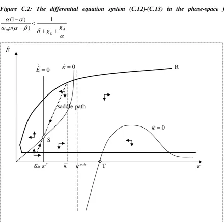
Definition 1: A partially balanced growth path (PBGP) is an equilibrium growth path where

aggregates (Y, K and E) grow at a constant rate.

Note that this definition does require balanced growth for aggregate variables. However, it

does not require balanced growth for subsectoral variables (e.g. for subsectoral outputs).

Lemma 1: When α , β , and are assumed to be exogenous and constant, equations

(22) to (24) imply that there exists a unique PBGP, where aggregates (Y, K, and E) grow at

constant rate and where is constant. The PBGP-growth rate is given by

A

g g_B

*

g lm/km

L A

g g

g = +

α

*

.

Proof: is self-evident.

Lemma 2: a) A saddle-path, along which the economy converges to the PBGP, exists in the

neighborhood of the PBGP. b) The PBGP is locally stable.

Lemma 2 ensures that, if a technological breakthrough shifts the economy away from the

PBGP, the economy will converge to the PBGP again, provided that the departure from the

PBGP is not too strong.

Lemma 3: Along the PBGP, labor is not reallocated betwee sectors A and B. That is, labor is

not reallocated across technology, i.e. l_A and l_B are constant.

Proof: This lemma is implied by equations (20) and (21) and by Lemma1. Q.E.D.

Note, however, that it can be easily shown that labor is reallocated within each of the sectors

A and B. Furthermore, note that in section 5 we will allow for labor reallocation between

sectors A and B.

4 Impacts of a technological breakthrough: self-reinforcing

technology-convergence/divergence

Now we study how a technology breakthrough affects the situation described in the previous

section. We assume an initial situation where the technologies differ across sectors.

As discussed in section 2.4, we assume that a technology breakthrough induces a finite period

of time where the breakthrough is implemented. During this period of implementation, the

sectoral technologies change. When the implementation-period is finished, the economy

converges to the new PBGP.4

As we will show now, the change in sectoral technologies during the implementation-period

leads to a change of cross-technology factor-allocation ( , ). The change in this allocation

affects the ability of the sectors to implement the next breakthrough (see e.g. section 2.4.4).

Hence, over time (and over a sequence of breakthroughs) the sectoral technologies may

converge or diverge over time.

A

l l_B

We will elaborate now the factors that determine whether the technologies converge or

diverge. To do so we calculate the employment shares along the PBGP. By using equations

(20)/(21) and some of the equations from APPENDIX we obtain the following employment

shares along the PBGP:

4

(25)

ρ α

δ ρ α ω α β

ρ α

δ ρ α α β

A L B

A L

B

g g

g g

l

+ + + + −

+ + + + − =

) (

1 *

(26) l_A* =1−l_B*

An asterisk denotes here the PBGP-value.

These equations imply that:

(27) 0 0

* *

< ∂ ∂ >

∂ ∂

β

βB A

l l

(28) 0 0

* *

> ∂ ∂ <

∂ ∂

α

αB A

l l

Note that in the calculation of (28), we assumed that an increase in α is associated with an

increase in gA, such that gA/α increases if α increases, according to our discussion in point

2) of Assumption 13.

Now we can postulate the following:

Theorem 1: Implementation of breakthroughs leads to a change in the PBGP-values of the

employment-shares of sectors A and B ( and ). That is, implementation of breakthroughs

leads to cross-technology labor-reallocation.

A

l lB

Proof: This theorem is implied by equations (27)/(28) and Assumption 13. Q.E.D.

Note that this theorem holds even if implementation is such that α and β increase by the

same amount. The reason is the following: a change in α and/or β leads to a change in

average economy-wide output-elasticity of labor; i.e. the average capital-intensity of the

economy (K/L) changes (as implied by Lemma 1). Since sector A (and especially subsector

m) produces capital, a change in average capital intensity affects the employment-share of

sector A, ceteris paribus. (See also equations (20) and (21) and note that aggregate investment

is equal to Y −E).

Of course in general, the change in and does not only come from this change in

aggregate capital demand. Additionally, the following fact determines the allocation ( , ):

A

l l_B

A

Optimal factor-allocation across sectors is determined by the profitability of factor-inputs in

sectors, since we assume perfect factor mobility across sectors. That is, sectors, which have

relatively high output-elasticity of labor, employ more labor in comparison to sectors, which

have relatively low output-elasticity of labor. (Previously, this fact has been shown by

Acemogly and Guerrieri (2008) in another model.) Therefore, a change in cross-sector

technology-bias (

β α

) induces an adjustment of input-shares, such that optimal

factor-input-shares are achieved. To understand this fact, note that equations (20) and (21) imply that

a change in

β α

induces a change in (l_A, lB) even if we keep lm/km, E and Y constant.

Hence, we can postulate the following corollary:

Corollary from Theorem 1: The change in cross-technology labor allocation ( , ), which

has been postulated in Theorem 1, comes from two forces:

A

l l_B

1.) A change in sectoral output-elasticities of inputs affects the aggregate capital demand;

since only sector A produces capital, the changes in aggregate capital demand induce

factor-reallocation across sectors A and B.

2.) A change in cross-sector technology-bias (α/β) changes the optimal factor-allocation

across sectors. Thus, when there is free factor-mobility across sectors, cross-sector factor

reallocations are induced in order to achieve the new optimal cross-sector factor allocation.

Theorem 1 is the basis for technology convergence and divergence, since cross-sector

labor-reallocation changes the sector’s relative potential to implement future breakthroughs

(according to Assumption 13).

According to the discussion in section 2.4.4 we distinguish between two cases.

1.) Implementation is labor-augmenting

According to our discussion in section 2.4.4 and equations (27)/(28) we can postulate the

following causal chain: A breakthrough leads to implementation in sector A (B), which

leads to increase in α (β), which leads to increase in ( ), which leads to better

implementation of the next breakthrough.

L l_A l_BL

2.) Implementation is capital-augmenting

According to our discussion in section 2.4.4 and equations (27)/(28) we can postulate the

leads to a decrease in α (β), which leads to a decrease in ( ), which leads to

weaker implementation of the next breakthrough.

L l_A l_BL

Hence, we can postulate the following theorem:

Theorem 2: a) If implementation is labor-augmenting, the implementation of a breakthrough

in sector A (B) increases the employment-share of sector A (B). If implementation is

capital-augmenting, the implementation of a breakthrough in sector A (B) reduces the

employment-share of sector A (B).

b) If implementation is labor-augmenting, the implementation of a breakthrough in sector A

(B) increases the ability of sector A (B) to implement the next breakthrough. If implementation

is capital-augmenting, the implementation of a breakthrough in sector A (B) reduces the

ability of sector A (B) to implement the next breakthrough.

Proof: This theorem is implied by equations (27)/(28) and Assumptions 12 and 13. Q.E.D.

Definition 2: Technology-bias is defined as α−β . The higher α−β , the stronger

technology-bias.

Theorem 3: Provided that there is a sequence of technological breakthroughs over a period

of time, the following factors jointly determine whether technology-bias decreases or

increases over this period of time:

a) the sort of implementation of technological breakthroughs (labor-augmenting vs.

capital-augmenting implementation)

b) the magnitude of the increase in (productivity) growth rate of capital-goods

production (g_A/α ), which is induced by the implementation of the breakthroughs

c) the sectors in which the breakthroughs are implemented (implementation in sector A,

sector B or in both sectors)

d) the correlation between sector size (l_A,l_B) and sector technology (α,β )

e) the difference between sector sizes (l_A−l_B).

Proof: First, we prove this theorem for a special case; then we argue that this proof can be

generalized. We first assume a reference case and then show the differences to this reference

case.

Reference case: Assume that . Furthermore assume that there is a breakthrough which

is implemented in both sectors in labor-augmenting manner. According to Assumption 13, the

B A l

increase in α (Δα) is larger than the increase in β (Δβ), i.e. Δα >Δβ, where Δα >0 and

0

>

Δβ . Hence, if α >β before implementation, the technology-bias (α −β ) is increased

by implementation.

Proof of part a): In contrast to the Reference case, assume that there is a breakthrough which

is implemented in both sectors in capital-augmenting manner, ceteris paribus. Thus,

according to Assumption 13, α decreases more strongly than β does, i.e. Δα > Δβ , where

0

<

Δα and Δβ <0. Hence, if α >β before implementation, the technology-bias (α β s

reduced by implementation, in contrast to the reference case. This fact proves part a) of

Theorem 3.

− ) i

Proof of part c): In contrast to the Reference case, assume that there is a breakthrough which

is implemented in labor-augmenting manner in sector B only, ceteris paribus, i.e. Δα =0 and

0

>

Δβ . Hence, if α >β before implementation, the technology-bias (α−β ) is reduced by

implementation, in contrast to the reference case. This fact proves part c) of Theorem 3.

Proof of part d): In contrast to the Reference case, assume that α <β before implementation,

ceteris paribus. In this case, technology-bias is reduced by implementation, in contrast to the

Reference case. This fact proves part d) of Theorem 3.

Proof of part b): Now assume the same situation as in the reference case. As shown there, the

implementation of the breakthrough increases α and β, i.e. Δα >0 and Δβ >0. Equations

(27)/(28) imply that these increases change the labor-allocation ( ). If this reallocation

process is such that becomes smaller than , the implementation of the next breakthrough

will yield mirror-image effects on the technology-bias in comparison to the initial reference

case. That is, this second breakthrough is implemented more strongly in sector B, which

would reduce the technology-bias. Now, the question is, under which circumstances is the

reallocation process, which is induced by the first breakthrough, such that becomes smaller

than . This can only happen if

B A l

l ,

A

l l_B

A

l

B

l

α

β ∂

∂ > ∂

∂lB lA

, where lA+lB=1. 5

In this case it can happen that

the changes in employment shares overweight the changes in output-elasticities of capital (at

least after a long sequence of many breakthroughs) such that at some point of time

breakthroughs become better implementable in sector B. After some algebra it can be shown

5 If

α

β ∂

∂ ≤ ∂

∂l_B l_A

, cannot become smaller than during the implementation of the first breakthrough, since in this phase

A

l l_B

β α >Δ

Δ . That is, if

α

β ∂

∂ ≤ ∂

∂lB lA

that

α

β ∂

∂ > ∂l_B l_A

can be satisfied only if the change in

∂ gA/α , which is induced by the

implementation of the first breakthrough, is relatively small. (If gA/α is relatively large

α

β ∂

∂ < ∂l_B l_A

). Note that

∂ /α determines the PBGP-growth rate of capital-goods-production,

Proof of part e): In the light of proof of part b) we can also postulate, th

A

g

since capital goods are produced in sector A only (see also Lemma 1).

at lA does not become

smaller than l_B during the first breakthrough, if the increase in g_A/α is r latively large (but

not too large) and the difference between l_A and l_B is rela large before the first

breakthrough. In this case, the fact that

e

tively

α

β ∂

∂ > ∂

∂lB lA _{cannot overweight the relatively strong}

difference between Δα and Δβ. Hence, the difference between and (i.e. the difference

is e s

nly valid in our

A

l lB

in implementability) decisiv for the development of the technology bia .

Note that it can be shown in analogous ways that Theorem 3 is not o

Reference case, but in all the other cases (e.g. if l_A <l_B). The proof of this fact is obvious. Q.E.D.

We discuss this theorem in Section 6.

The impacts of cross-technology structural change

res of (sub)sectors. That is,

chnology.

section we show that cross-technology structural change can affect the

technology-, Baumol (1967)technology-,

ge implies that structural change (across technology) is

caused by several determinants; especially, non-homothetic preferences (as modeled by

5

We define here structural change as changes in employment sha

we say that structural change takes place if (sub)sectoral employment shares change. It can be

easily shown that structural change takes place even along the PBGP in our model.

Cross-technology structural change means here that labor is reallocated across te

Hence, in our model, changes in (l_A,l_B) indicate that cross-technology structural change takes place.

In this

bias; i.e. structural change can lead to technology convergence/divergence.

Structural change is a well known fact and has been modeled by, e.g.

Kongamut et al. (2001), Ngai and Pissarides (2007), Acemoglu and Guerrieri (2008) and

Foellmi and Zweimueller (2008).

Kongsamut et al. 2001), cross-sector-differences in TFP-growth (as modeled by Ngai and

Pissarides 2007) and cross-sector-differences in capital-intensities (as modeled by Acemoglu

and Guerrieri 2008). Although all these determinants are included in our model, our

parameter-restriction (8c,d) prevent them from taking effect across technology; hence, l_A and

B

l are constant along the PBGP. Instead of deviating from parameter-restrictions (8c,d), which would make our analysis quite complicated, we model structural change as follows:

e assume that the utility-weights of technology change exogenously; i.e.

W ωB changes. This

leads to changes in demand and to structural change across technology. Hence, we do not

model the structural change (mentioned above) explicitly. Note that our way of modeling has,

in fact, very similar dynamic implications in comparison to the implications of structural

change models, which model the structural change determinants explicitly. In some sense, our

way of modeling only omits the microfoundations, which are anyway provided by the

previous literature.

Lemma 4: A onetime change in ω_B causes a deviation from the old PBGP and convergence to

e new PBGP.

eq th

Proof: This lemma is implied by uations (C.5) and Lemma 2. Q.E.D.

Theorem 4: a) A onetime increase in ω_B induces labor-reallocation from sector A to sector

, provided that

B α >β ; i.e. l_A decreases and l_B increases. b) A onetime increase in ω_B

induces labor-reallocation from sector B to sector A, provided that α <β; i.e. lA increases

and lB decreases.c) The stron er the difference b tween g e α and β, the stronger the change

in l_A and l_B. d) Analogous results are obtained for the case that ther onetime decrease

in

e is a

B

ω .

Proof: This lemma is implied by equation (25).

Corollary from Theorems 2, 3 and 4: Depending on the structural change pattern (i.e.

hether

w ω_B increases or decreases), structural change may lead to technology convergence

is simple: Structural change affects the employment

hare of a sector and thus sector’s ability to implement a breakthrough. For example, if the

income elasticity of demand of sector B is relatively high, factors are reallocated to sector B.

or divergence between sectors A and B.

In fact, the explanation of this corollary

This fact increases the ability of sector B to implement breakthroughs. Hence, if sector B was

technologically backward in the past, structural change (induced by income elasticity of

demand) may lead to technology convergence over time. This development may be reflected

by the reality: the backward sector B may be interpreted as the services sector (or at least as

some very labor-intensive subsectors of the services sector) that may catch up technologically

in future due to high income elasticity of demand.

By using similar arguments a case can be constructed where it may happen that technology

divergence occurs: if, e.g., income elasticity of demand of the technologically backward

sector is relatively low, technology divergence may be caused by structural change.

heorems 2, 3 and 4) we have

hown the relevance of several factors for the explanation of technology-bias:

(labor-augmenting vs.

capital-goods

See also the discussion in section 8 for some further arguments.

6 Summary of factors which determine technology-bias

In our model (especially in Theorem 3 and in Corollary from T

s

a) the sort of implementation of technological breakthroughs

capital-augmenting implementation)

b) the magnitude of the increase in the (productivity) growth rate of

production (g_A/α ), which is induced by the implementation of breakthroughs

the sectors in which the breakthrough

c) s are implemented (implementation in sector A,

d)

sector B or in both sectors)

the correlation between sector size (l_A,l_B) and sector technology (α,β )

e) the difference between sector sizes (lA−lB).

structural change f)

No arding the question why these factors affect the

dev p y-bias:

rogress reduces the optimal capital-intensity. Hence, the

ectors, which implement the breakthroughs, have to increase their labor input in order to w we provide intuitive explanations reg

elo ment of technolog

a.) The reasons for the relevance of the sort of implementation are the following: In general,

labor-augmenting technological p

s

profit from the implementation. However, in contrast to capital, labor cannot be accumulated;

hence, the sectors, which implement the breakthrough, pull labor from sectors, which do not

sectors than in small sectors6, labor is withdrawn from small sectors and reallocated to large

sectors. This fact reduces the ability of small sectors to implement future breakthroughs (less

creative potential). In contrast, capital-augmenting implementation increases the capital

intensity. Hence, big sectors can release some part of their labor-force, since it can be

substituted by capital (which can be accumulated endogenously). This labor-force is

reallocated to small sectors, which increases their creative potential and thus ability to

implement future breakthroughs. (See also the Corollaries from Theorems 1 and 2.)

b.) If productivity of capital-goods-production is increased by implementation of

reakthroughs, factors are reallocated to the sector, which produces capital. This

factor-s but factor-seemfactor-s to be relatively important. For example, if

reakthroughs are such that they can only be implemented in the progressive sector,

some mechanisms, which

orrelate the employment share with the output-elasticity of labor (see Theorem 2), it is

b

reallocation affects the ability of these sectors to implement future breakthroughs. Thus, the

development of the technology bias is affected by this fact. This effect arises only if

capital-goods-production is not evenly distributed across all sectors. In our model this is the case:

only sector A produces capital-goods. (Thus, the productivity of sector A corresponds to

productivity of capital-goods-production.) Empirical evidence implies that this assumption is

preferable: e.g. in the USA, capital-goods are produced primarily by the manufacturing sector

and output-elasticity of capital differs across consumption-goods and capital-goods; see e.g.

Valentinyi and Herrendorf (2008).

c.) This point is relatively obviou

b

technology-bias increases. It may be possible that nature of the development-process is such

that it features different phases, where in early phases some breakthroughs occur which can be

implemented primarily in manufacturing and where in later phases breakthroughs occur,

which can be implementation in some (personal) services sectors.

d.) Despite of our model results, which postulate that there are

c

possible to deviate from this scheme. For example, we have shown in the previous section that

income elasticity of demand may cause deviations from this scheme. Hence, it is possible that

large sectors (large employment shares) are associated with low output-elasticity of labor, if

their income elasticity of demand is relatively large. The fact, that the correlation between

6

employment share and output-elasticity may be important regarding the technology-bias, is

relatively obvious: If progressive sectors have high employment shares (negative correlation

between output-elasticity and employment shares), implementation in progressive sectors is

more successful than in implementation in backward sectors, hence technology-bias increases.

Otherwise, if progressive sectors have low employment shares (positive correlation),

implementation will be less successful, and backward sectors catch up (technology-bias

decreases).

e.) We assume that the difference in sector size determines how strong the difference in

plementation of breakthroughs across sectors is. If there are very small sectors and very

section, structural change is caused by several determinants.

ence, all these determinants affect the cross-sector-factor allocation and thus relative

d here, but

hich affect the model outcome. These factors rather depend on the nature of the

e of the breakthrough whether it is

implement the same

sector; which would yield technology im

large sectors in an economy, the differences in technology are large (according to our model)

and may be difficult to overweight by other effects (e.g. those from point b)), as seen in the

proof of Effect b) in Theorem 3.

f.) As mentioned in the previous

H

abilities to implement breakthroughs. For further discussion see previous section.

Last not least, there are several further factors, which are not explicitly modele

w

breakthrough and/or on the nature sectoral output. Some discussion of the nature of sectors

and its implications for the scope of technological progress can be found, e.g. in the essays by

Wolfe (1955), Baumol (1967) and Klevorick et al. (1995).

1.) It may happen that some breakthroughs are rather implementable in capital-augmenting or

labor-augmenting way. That is, it may depend on the natur

primarily labor-augmentingly or capital-augmentingly implemented.

2.) Some sectors (e.g. services) may implement a breakthrough (e.g. electricity) in a primarily

labor-augmenting way and other sector (e.g. agriculture) may

breakthrough (electricity) in a primarily capital-augmenting way. This could yield

technology-divergence. That is, in which way the breakthroughs are primarily implemented

may depend on the nature of the output of a sector.

3.) Simply speaking, it may also be accidental that over some period of time breakthroughs

convergence. As well technical feasibility may dictate the order of breakthroughs and thus

development of the technology-bias.

Overall, there seems to be some accidental or technical component which determines the

mely order of breakthroughs and their implementability in a sector.

Empirical evidence on technology convergence

this section we construct a simple measure of cross-sector technology-bias and analyze its

ral labor-income shares as ti

7

In

development over time. Since quite easy measurable, we use secto

indices of sectoral technology (output-elasticity of labor).

The measure of technology-bias, which we suggest is the following:

∑

⎠ ⎜⎜

⎝ − =

i i

t i i

l

Var₁

α α

⎞

⎛ 2

0 1 1

(29)

where

(30) ≡

∑

i t i i i

α l α

1

1 0

ernatively or alt

∑

= i

i

l

Var₂

(31) _⎟⎟

⎠ ⎞ ⎜⎜

⎝ ⎛

− i t i T

2

1 1

α α

(32) where

∑

≡

i t i T i i

α l α

1 1

i denotes sector; is the labor-income share of sector i at time t (or approximately

output-elasticity of labor); is the employment-share of sector i at time t; is the

variance-calculation, since

where αit

t i

l li0

employment-share of sector i at the beginning of the observation period; T is the

employment-share of sector i at the end of the observation period.

That is, our measure of cross-sector technology variation is simply a variance. Note that it

makes sense to use the employment-shares as weighting-factors in

i

l

it is theoretically reasonable:

wL Y wL

Y p L

wl Y p l

l i

i i i

i i

i = = =

i i i i

∑

∑

∑

. Hence, this term is equal

Note that we do not use the actual employment-shares to calculate the technology-variance,

m the beginning of the observation p

of the period.) The reason for

estic-Product-(GDP)-by-Industry-Data, which is based on the sector-definition

m data for longer

Industrial Classification System” has been

e (hence, the sector definition after 1987 is not the same as the sector

but the employment-shares fro eriod. (For control we also

calculate the variance by using employment-shares at the end

this is that the employment shares change over time and they would eventually bias the

technology development. Hence, with actual employment shares we could not say whether the

technology-variance decreased or whether some changes in employment-shares led to the

result.

For the calculations in this section I use the data for the U.S.A., which is available at the

web-site of the U.S. Department of Commerce (Bureau of Economic Analysis). I use the

U.S.-Gross-Dom

from the “Standard Industrial Classification System”, which defines the following sectors:

(1) Agriculture, forestry, and fishing

(2) Mining

(3) Construction

(4) Manufacturing

(5) Transportation and public utilities

(6) Wholesale trade

(7) Retail trade

(8) Finance, insurance, and real estate

(9) Services

My calculations are based on the data for the period 1948-1987. Unifor

periods is not available, since the “Standard

modified over tim

definition before 1987).

To calculate the sectoral labor-income-shares (α_i) I divide “(Nominal) Compensation of

Employees” by “(Nominal) Value Added by Industry” in each sector. The sectoral

employment shares (l_i) are calculated by using the sectoral data on “Full-time Equivalent

Employees”. (This approach is similar to that used by Acemogu and Guerrieri (2008)).

Both measures imply that the cross-sector technology-variance is decreasing. Hence, it seems

at technologies converged during the observation period.

ess has been capital-augmenting;

These explanations are discussed in the next chapter. th

In fact, our model-explanations of this finding are:

- Over the long-run in the past, technological progr

hence technologies are converging now.

- Structural change has increased the employment in technologically backward sectors