A Bivariate Chance Constraint of Wind Sources for Multi Objective Dispatching

A Bivariate Chance Constraint of Wind Sources for

Multi-Objective Dispatching

Mostafa Elshahed, Hussein Zeineldin, Magdy Elmarsfawy

Electrical Power and Machine Department, Faculty of Engineering, Cairo University, Cairo, Egypt. Email: [email protected]

Received May 5th_{, 2013; revised June 5}th_{, 213; accepted June 14}th_{, 2013}

Copyright © 2013 Mostafa Elshahed et al. This is an open access article distributed under the Creative Commons Attribution License, which permits unrestricted use, distribution, and reproduction in any medium, provided the original work is properly cited.

ABSTRACT

The economic emission dispatch (EED) problem minimizes two competing objective functions, fuel cost and emission, while satisfying several equality and inequality constraints. Since the availability of wind power (WP) is highly de- pendent on the weather conditions, the inclusion of a significant amount of WP into EED will result in additional con- straints to accommodate the intermittent nature of the output. In this paper, a new correlated bivariate Weibull probabil- ity distribution model is proposed to analytically remove the assumption that the total WP is characterized by a single random variable. This probability distribution is used as chance constraint. The inclusion of the probability distribution of stochastic WP in the EED problem is defined as the here-and-now strategy. Non-dominated sorting genetic algorithm built in MATLAB is used to handle the EED problem as a multi-objective optimization problem. A 69-bus ten-unit test system with non-smooth cost function is used to test the effectiveness of the proposed model.

Keywords: Correlated Weibull Distribution; Economic Emission Dispatch; Stochastic Programming; Wind Power

1. Introduction

Wind energy is the most attractive clean and fuel-free solution to the world’s energy challenges. Well estab- lished in more than 50 countries all over the world, sup- plying more than 250 GW as total installed capacity and forecasted to provide 30% of the world’s electricity by 2030 [1]. One of the challenges is how to appropriately characterize Wind Power (WP) in the load dispatch model. A conventional economic dispatch problem uses deterministic models, which can not reflect situations considering the WP injection. Since wind farms con- nected to power systems have characteristics of dynamic and stochastic performance, stochastic models are more suitable. There are several studies intended to investigate the injection of WP into conventional power networks and its impact on the generation resource management due to its stochastic and non-dispatchable characteristics. A conventional way was to use the average WP. The probabilistic conventional approaches tried to find prob- abilistic characteristics of solutions of the problem under investigation [2-8]. This approach is called the wait-and- see (WS) strategy in the context of stochastic program- ming. Although these approaches can be easily imple- mented, it has a less-known pitfall, called the probabilis-

tic infeasibility. The probabilistic feasibility of the aver- age WP is 0.25, or equivalently, the probabilistic infeasi- bility is as large as 0.75 [8,9].

For this reason, one of the more appropriate strategies in contrast, the here-and-now (HN) strategy introduces the probabilistic characteristics to the model of optimiza- tion problem itself. A here-and-now model of a power system with wind energy generators was developed [10-13]. The authors introduced the stochastic distribu- tion of wind speed into the economic dispatch issue con- sidering both reserve cost of overestimation and penalty cost of underestimation of available wind power. The scheduled wind power output was an estimation value of available wind power output and it was treated as an op- timization variable, which was dependent on several fac- tors such as the reserve cost and the penalty cost. But these costs are very difficult to be exactly determined [10].

tolerance that the total load demand cannot be satisfied. Choosing small pa will mitigate the risk of insufficient WP, while increasing the demand for thermal power.

To analytically remove the assumption that the total WP is characterized by a single random variable, the correlated Weibull distribution (Multivariate Distribu- tions according to Probability Theorems) of the sum of WP is derived from the Weibull distribution model of each WP cluster. This correlated Weibull distribution is used as a chance constraint in the proposed model. With increasing concern over global climate change, policy makers are promoting renewable energy sources, predo- minantly wind generation, as a means of meeting emis- sions reduction targets. Although wind generation does not itself produce any harmful emissions, its effect on power system operation can actually cause an increase in the emissions of conventional plants [18]. Thus, the eco- nomic dispatch problem can be handled as a multiob- jective optimization problem with non-commensurable and contradictory objectives.

In this paper, an EED model is developed for the system consisting of both thermal generators and wind turbines with more realistic and practical considerations. A nondominated sorting genetic algorithm based appro- ach was used for solving the proposed EED model. The problem was formulated as a nonlinear constrained multi-objective optimization problem where fuel cost and environmental impact are treated as competing objectives. Two runs were carried out on a standard test system with non-smooth cost function and the results are analyzed and compared to those of previous works. The effecti- veness and potential of the proposed multi-objective EED model are demonstrated.

2. Economic Emission Dispatch Model

The EED problem is to minimize two competing objec- tive functions, fuel cost and emission, while satisfying several equality and inequality constraints. Generally the problem is formulated as follows.

2.1. Objective Functions  Minimization of Fuel Cost:

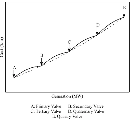
In the past, to solve economic dispatch problem effec- tively, most algorithms require the incremental cost curves to be of monotonically smooth increasing nature and continuous. The generating units with the multi- valve steam turbines exhibit a greater variation by the fuel-cost functions, where the valve point results in the ripple form of the heat-rate curve and the cost function contains higher order nonlinearity due to the valve-point effects, as shown in Figure 1. The more general fuel cost

function of each thermal generator considering the valve- point effect in terms of real power output is expressed as

Generation (MW)

A: Primary Valve B: Secondary Valve C: Tertiary Valve D: Quaternary Valve

E: Quinary Valve

Co

st

(

$/

hr

)

E

D

C B

[image:2.595.313.535.85.287.2]

A

Figure 1. Non-smooth cost function with five valves.

the sum of a quadratic and a sinusoidal function as fol- low [16]:

 

2









,min sin

i i i i i i i i i i i

C p  a b P c P d e P P (1)

 Minimization of Emission:

The atmospheric pollutants such as sulphur oxides (SOx) and nitrogen oxides (NOx) caused by conventional thermal units can be modeled separately. However the total emission of these pollutants which is the sum of a quadratic and an exponential function can be expressed as [19]:

 

2 _exp



i i i i i i i i i i

E p   P P   P



N

(2)

2.2. Real Power Operating Limits

,min ,max; 1, 2, ,

i i i

P P P i  (3)

2.3. Stochastic Chance Constraint

The power balance constraint is expressed as following:

Losses N

i d

i

P W P P



(4) In chance-constrained programming in the context of stochastic programming, the probability distribution functions of the random variables are used as constraints in the optimization problem. The main goal with chance constraints is, therefore, to determine deterministic equi- valents [20]. If the total WP is characterized by a single random variable, the stochastic WP constraint and power balance constraint can be expressed as following [9,14- 16]:

 

Losses

Pr N _{i d}

i

P W P P

 

a

p

    

 

In particular, a threshold parameter pa is introduced into the constraint to characterize the tolerance that the total load demand cannot be satisfied [9]. Choosing small pa will mitigate the risk of insufficient WP, while in- creasing the demand for thermal power. Using Weibull PDF of wind power (5) will be:

 

 





Pr Pr 1 exp 1 exp M

i d Losses

i

M d Losses i

i k

out

k M

in r r in d i

k k

i r

p W P P

W P P p

v c

v w v v P p

w c  _{   }         _    _    _{ }    _{ }         _{  }     _ _   _  _{ }        







(6)

This assumes that all wind turbines are located in a coherent geographic area. To analytically remove this assumption, the correlated Weibull distribution is needed. Practically, a large wind farm can be divided into multi- ple clusters. Hence, from the Weibull distribution model of each cluster, the correlated Weibull distribution of the sum of WP will be derived to be used in proposed mod- els in the next section. For simplification, we only start with two random variables. It implies that we assume that total WP is characterized by two random variables or that wind turbines are located in two different geographic areas.

3. The Correlated Distribution Function

Often an experiment involves measuring two or more random numbers, say X and Y. The fact that we know the distribution of X, and the distribution of Y separately doesn’t determine probabilities of events that involve both X and Y simultaneously [21]. The distribution func- tions FX(x) and FY(y) of the given random variables de- termine their separate (marginal) statistics but not joint statistics simultaneously [22].

3.1. Joint Cumulative Distribution and Probability Distribution Functions

The joint (bivariate) cumulative distribution function (CDF) FXY (x, y), or simply, F (x, y) of two random vari- ables X and Y is the probability of the event [22]:

 

, Pr





Pr



  

, ,

XY

F x y  X x  Y y  x y D (7)

The joint probability distribution function (PDF) of X

and Y is by definition [22]:

 

, 2F x y

 

,

f x y

x y  

  (8)

3.2. One Function of Two Random Variables

Given two random variables X and Y with Z is the sum of them, we want to find the random variable Z joint statis- tic probability distributions [21].

 The Joint CDF is obtained as following:

 

z-y

 

, d d Z

F z f x y



 



_{ }

x y (9)

 And Joint PDF is obtained as following:

 





, d Z

f z f z y y 





_

 y



(10)

 Statistically Independent Events and Convolution:

If X and Y are statistically independent then:

 



  







-d

Z X Y X Y

f z f z y f y y f z y f y 





_

    (11)

where :Convolution

If two random variables are independent, then the PDF of their summation equals the convolution of their PDF [21].

3.3. Bivariate PDF of WP with Two Weibull Random Variables

Since the probability distribution of the WP random variable Wi:

 

























, , , , 1 , , , , , , , , 1 1 1 1 1 exp i i i i i r i in i in

W i

i r i

k i r i in i

i in i r

i

k i r i in i

i in i r

i

k v v v

f w

w c

v v w

v w

c

v v w

v w c         _   _ _             _{   }   _{   }   _{  }   _  _   _ _    _{ }   _{ }   _{ }    (12)

Hence the joint statistic probability distributions of random variable W, where W is the sum of two random variables W1 and W2, is:

 





 





 

1 2 1 2 2 2 -2 2 d

W W W

W W

2

f w f w w f w

f w w f w

      



w (13)

 

0

Pr d

X N

d Losses i W a

i

W P P P f w w p

 _ _{ } _{ }

  

 









(14)

where: _{d Losses} N _i

i

X P P 



P

All integrations, differentiations, and convolution op- erations required in the previous derivation or in the op- timization problem solution are executed by using the symbolic MuPAD built in MATLAB.

Hence the economic emission dispatch model can be mathematically formulated as follows:

 









 





2

,min

1 1

2

1 1

Minimize :

sin

exp

N N

i i i i i i i i i i i

i i

N N

i i i i i i i i i i

i i

C p a b P c P d e P P

E p  P  P   P

 

 

 _{    }

 

 _{   }











Subject to: Pi,min PiPi,max

 

0

Pr d

X N

d Losses i W a

i

W P P P f w w p

 _ _{ } _{ }

 _ _









This model, referred to as the here-and-now approach, avoids the probabilistic infeasibility appearing in con- ventional models and used the derived correlated Weibull distribution of the sum of WP as constraint to avoid the assumption that the total WP is characterized by a single random variable. The transmission losses in terms of B-coefficients in the power balance constraint and more practical cost functions for thermal units were considered in the proposed model.

4. Results and Discussion

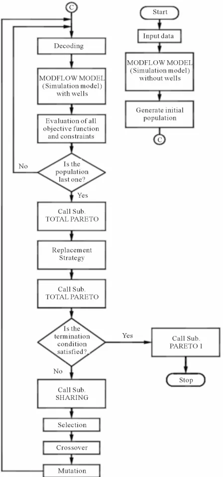
The practical EED problems have non-smooth cost func- tions with equality and inequality constraints in addition to the wind power chance constraint that make the prob- lem of finding the global optimum difficult using any mathematical approaches, so a numerical optimization procedure is needed. In this paper, therefore, we imple- mented the nondominated sorting multi-objective genetic algorithm in MATLAB to deal with proposed model, the flow chart can be found in the Appendix B [23]. A 69-

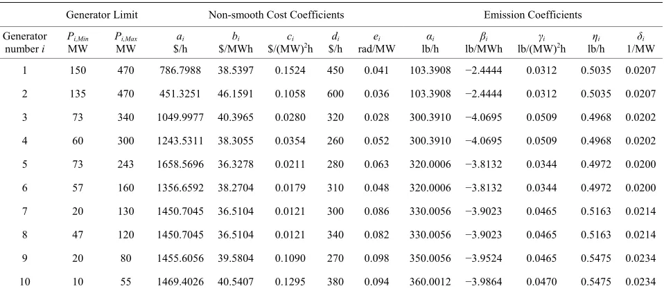
bus ten-unit test system with non-smooth fuel cost func- tion is used in this paper to demonstrate the performance and the effectiveness of proposed model. Thermal units’ data was taken from [24] and can be found in Appendix C.

Kalyanmoy introduced full details about Multi-objec- tive Genetic Algorithm, but are beyond the scope of dis- cussion here [25]. The proposed model was tested with the 69-bus 10-unit at forecasted load 1800 MW. Thre- shold parameter pa = 0.4. The Pareto front population fraction was considered in two different cases as follow:

 Case (1) with Pareto front population fraction = 0.7.  Case (2) with Pareto front population fraction = 0.35.

Figures2 and 3 show a set of nondominated optimal

Pareto solution of the proposed model with Pareto front population fraction 0.7 and 0.35, respectively. As shown in Figures2 and 3, there is no single solution that is op-

timal with respect to all objectives of the multi-objective optimization problem. Instead, there is a set of solutions that are superior to the rest of the solutions in the search space considering all objectives. Further, there is no so- lution in this set is absolutely better than the other solu- tions. This set is called the Pareto optimal set. It can be seen that the most left side Pareto solution of Figures 2

and 3 gives the Pareto solution of the minimum fuel cost

and the most right side Pareto solution of Figures 2 and 3 denotes the Pareto solution of the minimum emission.

[image:4.595.66.285.231.349.2]

Also, there is the Pareto solution that means the turning point of a set of optimal Pareto solutions.

Figure 2. The set of Pareto solutions of the proposed system Case 1.

[image:4.595.309.536.531.702.2]

Area A shows the Pareto solutions that emphasize the economy, while the area B gives the Pareto solutions that emphasize the environmental protection. Table 1 gives

values of objective functions and the generators outputs for solutions S, T and U in Figure 2 with Pareto front

population fraction 0.7. Table 2 gives values of objective

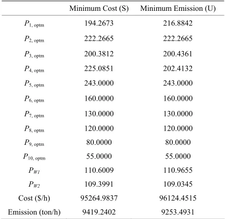
[image:5.595.55.288.244.474.2]

functions and the generators outputs for minimum fuel cost and minimum emission with Pareto front population fraction 0.35 at the most left side and the most right side of Figure 3, respectively.

Table 1. The objective functions and the generators outputs for Case 1.

Minimum Cost (S)

Middle (T)

Minimum Emission (U)

P1, optm 216.6096 226.4008 235.2070

P2, optm 216.8540 225.1419 233.5409

P3, optm 215.1373 207.2091 201.6535

P4, optm 217.8698 210.6210 202.3924

P5, optm 219.5344 218.3747 217.3775

P6, optm 159.9989 158.7998 157.5778

P7, optm 129.9989 129.2052 128.1667

P8, optm 119.9996 119.8012 119.4389

P9, optm 79.9989 79.4731 79.7809

P10, optm 53.9970 54.9721 54.8632

PW1 110.0158 110.0454 110.2052

[image:5.595.57.286.513.736.2]

PW2 109.9852 109.9553 109.7958 Cost ($/h) 96047.7637 96725.1128 97916.7323 Emission (ton/h) 9414.4405 9328.6960 9282.2429

Table 2. The objective functions and the generators outputs for Case 2.

Minimum Cost (S) Minimum Emission (U)

P1, optm 194.2673 216.8842

P2, optm 222.2665 222.2665

P3, optm 200.3812 200.4361

P4, optm 225.0851 202.4132

P5, optm 243.0000 243.0000

P6, optm 160.0000 160.0000

P7, optm 130.0000 130.0000

P8, optm 120.0000 120.0000

P9, optm 80.0000 80.0000

P10, optm 55.0000 55.0000

PW1 110.6009 110.9655

PW2 109.3991 109.0345 Cost ($/h) 95264.9837 96124.4515

Emission (ton/h) 9419.2402 9253.4931

In Figure 2, it can be seen that the Pareto solution of

solution U succeeds in reducing 1.42% of amount of emission and degrading 1.95% of the fuel cost in com- parison with solution S. In addition, solution T succeeds in reducing 0.93% of amount of emission and degrading 0.71% of the fuel cost in comparison with solution S.

Table 1 also shows outputs of generators in Pareto solu-

tions. It can be seen that 1st and 2nd generators have low emission output and high fuel cost because their powers are increasing from solution S to solution T to solution U. Case 1, with Pareto front population fraction 0.7, pre- serves the diversity of the nondominated solutions over the trade-off front and solve effectively the problem.

The results of the proposed EED model were com- pared to previous work [15] which obtained the effect of emission constraint and representation of losses. It can be seen that the minimum fuel cost in the proposed model is more than that by Elshahed et al. [15] without consider- ing emission constraint by about 1.9 % and the savings with the proposed model in fuel cost are about 1.4 % when the emission constraint is considered by Elshahed

et al. [15]. In addition, the proposed model gives more efficient and noninferior solutions of multi-objective optimization problems.

In contrast with single objective optimization problem found by Elshahed et al. with emission constraint [17], the single solution that is optimal with respect to all ob- jectives of the multi-objective optimization problem does not exist. Instead, there is a set of solutions that is supe- rior to the rest of the solutions in the search space con- sidering cost and emission objectives, so there is no solu- tion in this set is absolutely better than the other solutions. The final decision will be taken by the system dispatch- ers according to the dispatcher’s attitude. The considered model in this paper achieved saving in minimum fuel cost about 5.8 % when compared with that with single objective function and emission constraint [17]. It can be seen that the wind power results in all solutions are al- most constant, because the wind units’ parameters are not changed and also the two units are identical.

5. Conclusions

In this paper, an accurate multi-objective EED model is presented including:

 The transmission losses in terms of B-coefficients,  Non-smooth cost functions due to valve-point effect,

and

 The correlated Weibull probability distribution of the WP constraint for a system consisting of both thermal generators and wind turbines.

the risk due to uncertainty and can result in minimizing the required spinning reserve. Hence this model is more realistic, practical, and accurate economic emission dis- patch model.

In addition, the nondominated solutions in the ob- tained Pareto-optimal set are well distributed and have satisfactory diversity characteristics which give informa- tion regarding the available trade-offs to the system op- erators. Finally, we can conclude that the proposed EED model provides valuable information and suggestions for safe, reliable, and economic operation of power systems. The results obtained provide direct guidelines for system operators to make correct decisions to schedule the sys- tem with WP.

6. Acknowledgements

The authors gratefully acknowledge Dr. Hatem Zeineldin for his guidance and unlimited support during this work.

REFERENCES

[1] http://www.wwindea.org/home/index.php

[2] P. Zhang and S. T. Lee, “Probabilistic Load Flow Com- putation Using the Method of Combined Cumulants and Gram-Charlier Expansion,” IEEE Transactions on Power Systems, Vol. 19, No. 1, 2004, pp. 676-682.

doi:10.1109/TPWRS.2003.818743

[3] A. Schellenberg, W. Rosehart and J. Aguado, “Cumulant- Based Probabilistic Optimal Power Flow (P-OPF) with Gaussian and Gamma Distributions,” IEEE Transactions on Power Systems, Vol. 20, No. 2, 2005, pp. 773-781.

doi:10.1109/TPWRS.2005.846184

[4] A. Schellenberg, W. Rosehart and J. Aguado, “Introduc- tion to Cumulant-Based Probabilistic Optimal Power Flow (P-OPF),” IEEE Transactions on Power Systems, Vol. 20, No. 2, 2005, pp. 1184-1186.

doi:10.1109/TPWRS.2005.846188

[5] D. Villanueva, A. Feijóo and J. Luis Pazos, “Probabilistic Load Flow Considering Correlation between Generation, Loads and Wind Power,” Smart Grid and Renewable En- ergy, Vol. 2, No. 1, 2011, pp. 12-20.

doi:10.4236/sgre.2011.21002

[6] Q. Fu, D. C. Yu and J. Ghorai, “Probabilistic Load Flow Analysis for Power Systems with Multi-correlated Wind Source,” Power and Energy Society General Meeting, San Diego, 24-29 July 2011, pp. 1-6.

doi:10.1109/PES.2011.6038992

[7] H. Yang and B. Zou, “The Point Estimate Method Using Third-Order Polynomial Normal Transformation Tech- nique to Solve Probabilistic Power Flow With Correlated Wind Source and Load,” Asia-Pacific Power and Energy Engineering Conference (APPEEC), Shanghai, 27-29 March 2012, pp. 1-4.

doi:10.1109/APPEEC.2012.6307479

[8] X. Liu, “Economic Load Dispatch Constrained by Wind Power Availability: A Wait-and-See Approach,” IEEE Transactions on Smart Grid, Vol. 1, No. 3, 2010, pp. 347-

355. dio:10.1109/TSG.2010.2057458

[9] X. Liu and W. Xu, “Economic Load Dispatch Constrain- ed by WP Availability: A Here-and-Now Approach,” IEEE Transactions on Sustainable Energy, Vol. 1, No. 1, 2010, pp. 2-9. doi:10.1109/TSTE.2010.2044817

[10] J. Hetzer and D. C. Yu, “An Economic Dispatch Model Incorporating Wind Power,” IEEE Transactions on En- ergy Conversion, Vol. 23, No. 2, 2008, pp. 603-611.

doi:10.1109/TEC.2007.914171

[11] D. Villanueva, A. Feijóo and J. Pazos, “Simulation of Correlated Wind Speed Data for Economic Dispatch Eva- luation,” IEEE Transactions on Sustainable Energy, Vol. 3, No. 1, 2012, pp. 142-149.

doi:10.1109/TSTE.2011.2165861

[12] Y. Fang, D. Zhao, M. Ke, X. Zhao, C. Herbert and K. Wong, “Quantum-Inspired Particle Swarm Optimization for Power System Operations Considering Wind Power Uncertainty and Carbon Tax in Australia,” IEEE Trans- actions on Industrial Informatics, Vol. 8, No. 4, 2012, pp. 880-888. doi:10.1109/TII.2012.2210431

[13] G. S. Piperagkas, A. G. Anastasiadis and N. D. Hatziar- gyriou, “Stochastic PSO-Based Heat and Power Dispatch under Environmental Constraints Incorporating CHP and Wind Power Units,” Electric Power Systems Research, Vol. 81, No. 1, 2011, pp. 209-218.

doi:10.1016/j.epsr.2010.08.009

[14] X. Liu, W. Xu and C. C. Huang, “Economic Load Dis- patch with Stochastic Wind Power: Model and Solu- tions,” Transmission and Distribution Conference and Exposition, New Orleans, 19-22 April 2010, pp. 1-7.

doi:10.1109/TDC.2010.5484550

[15] M. Elshahed, M. Elmarsfawy and H. Zeineldin, “A Here-and-Now Stochastic Economic Dispatch with Non- Smooth Fuel Cost Function and Emission Constraint,” The Online Journal on Electronics and Electrical Engi-neering (OJEEE), Vol. 3, No. 4, 2011, pp. 484-489. [16] M. Elshahed, M. Elmarsfawy and H. Zeineldin, “Dyna-

mic Economic Dispatch Constrained by Wind Power Weibull Distribution: A Here-and-Now Strategy,” World Academy of Science, Engineering and Technology Jour- nal,Vol. 56, 2011, pp. 384-389.

[17] M. Elshahed, M. Elmarsfawy and H. Zeineldin, “A New Economic Dispatch Constrained by Correlated Weibull Probability Distribution Model for Wind Power,” IEEE PES Conference on Innovative Smart Grid Technologies- ME, Jeddah, 17-20 December 2011, pp. 1-6.

doi:10.1109/ISGT-MidEast.2011.6220811

[18] X. Liu and W. Xu, “Minimum Emission Dispatch Con- strained by Stochastic Wind Power Availability and Cost,” IEEE Transactions on Power Systems, Vol. 25, No. 3, 2010, pp. 1705-1713.

doi:10.1109/TPWRS.2010.2042085

[19] M. A. Abido, “Environmental/Economic Power Dispatch Using Multi-Objective Evolutionary Algorithms,” IEEE Transactions on Power Systems, Vol. 18, No. 4, 2003, pp. 1529-1537. doi:10.1109/TPWRS.2003.818693

Inc., Berlin, 2007.

[22] A. Papoulis, “Probability, Random Variables and Stocha- stic Processes,” 3rd Edition, McGraw-Hill Inc., Boston, 1991.

[23] T. A. Saafan, S. H. Moharram, M. I. Gad and S. K. Allah, “A Multi-Objective Optimization Approach to Ground- water Management Using Genetic Algorithm,” Interna- tional Journal of Water Resources and Environmental

Engineering, Vol. 3, No. 7, 2011, pp. 139-149.

[24] M. Basu, “Dynamic Economic Emission Dispatch Using Non-Dominated Sorting Genetic Algorithm-II,” Electri- cal Power and Energy Systems Journal, Vol. 30, No. 2, 2008, pp. 140-149. doi:10.1016/j.ijepes.2007.06.009

[25] K. Deb, “Multi-Objective Optimization Using Evolution- ary Algorithms,” John Wiley & Sons, Ltd., Chichester, 2001.

Appendix A

Nomenclatures

ai, bi, ci, di, and ei: Cost coefficients of ith unit αi, βi, γi, ηi, δi: Emission coefficients of ith _unit

c: Scale factor of the Weibull distribution

k: Shape factor of the Weibull distribution

N: Number of Thermal generators

Pi,min and Pi,max: Min and Max power generated by gen- erator i

Pi:Real power generated by generator i Pd:Total Load Demand

PLosses: Transmission System Losses Pr (E): Probability of event E Pd:Total Load Demand

PLosses: Transmission System Losses

pa: specified threshold representing the tolerance that the total demand cannot be satisfied.

vr, vin, and vout: Rated, cut-in, and cut-out wind speeds W:Real power generated by wind farm

wr:Rated wind power

(W): a Weibull PDF functional of random variable W

Appendix B

[image:7.595.312.537.237.716.2]

The flowchart of the multi-objective genetic algorithm used in this paper is shown in Figure 4.

[image:8.595.60.539.119.331.2]

Appendix C

Table C1. Conventional generators characteristics.

Generator Limit Non-smooth Cost Coefficients Emission Coefficients Generator

number i Pi,Min MW

Pi,Max MW

ai $/h

bi $/MWh

ci

$/(MW)2_{h $/h}di _rad/MWei _lb/h αi _lb/MWh βi _lb/(MW)γi 2_{h lb/h} ηi _1/MWδi

[image:8.595.49.540.361.410.2]

1 150 470 786.7988 38.5397 0.1524 450 0.041 103.3908 −2.4444 0.0312 0.5035 0.0207 2 135 470 451.3251 46.1591 0.1058 600 0.036 103.3908 −2.4444 0.0312 0.5035 0.0207 3 73 340 1049.9977 40.3965 0.0280 320 0.028 300.3910 −4.0695 0.0509 0.4968 0.0202 4 60 300 1243.5311 38.3055 0.0354 260 0.052 300.3910 −4.0695 0.0509 0.4968 0.0202 5 73 243 1658.5696 36.3278 0.0211 280 0.063 320.0006 −3.8132 0.0344 0.4972 0.0200 6 57 160 1356.6592 38.2704 0.0179 310 0.048 320.0006 −3.8132 0.0344 0.4972 0.0200 7 20 130 1450.7045 36.5104 0.0121 300 0.086 330.0056 −3.9023 0.0465 0.5163 0.0214 8 47 120 1450.7045 36.5104 0.0121 340 0.082 330.0056 −3.9023 0.0465 0.5163 0.0214 9 20 80 1455.6056 39.5804 0.1090 270 0.098 350.0056 −3.9524 0.0465 0.5475 0.0234 10 10 55 1469.4026 40.5407 0.1295 380 0.094 360.0012 −3.9864 0.0470 0.5475 0.0234

Table C2. Two wind units parameters.

Unit No. k c (m/sec) vin (m/sec) vout (m/sec) vr(m/sec) wr (pu)

1 1.7 15 5 45 15 150

2 1.7 15 5 45 15 150

The Transmission Losses Coefficients:

0.000049 0.000014 0.000015 0.000015 0.000016 0.000017 0.000017 0.000018 0.000019 0.000020 0.000014 0.000045 0.000016 0.000016 0.000017 0.000015 0.000015 0.000016 0.000018 0.000018 0.000015 0.000016 0.000039 0.000010 0.0000

B

12 0.000012 0.000014 0.000014 0.000016 0.000016 0.000015 0.000016 0.000010 0.000040 0.000014 0.000010 0.000011 0.000012 0.000014 0.000015 0.000016 0.000017 0.000012 0.000014 0.000035 0.000011 0.000013 0.000013 0.000015 0.000016 0.000017 0.000015 0.000012 0.000010 0.000011 0.000036 0.000012 0.000012 0.000014 0.000015 0.000017 0.000015 0.000014 0.000011 0.000013 0.000012 0.000038 0.000016 0.000016 0.000018 0.000018 0.000016 0.000014 0.000012 0.000013 0.000012 0.000016 0.000040 0.000015 0.000016 0.000019 0.000018 0.000016 0.000014 0.000015 0.000014 0.000016 0.000015 0.000042 0.000019 0.000020 0.000018 0.000016 0.000015 0.000016 0.000015 0.000018 0.000016 0.000019 0.000044

 

 

 

 

 

 

 

 

 

 

 

 

 

 

 