An Endowment Effect for Risk:
Experimental Tests of Stochastic Reference Points
∗
Charles Sprenger
†University of California, San Diego
September, 2010
This Version: January 14, 2011Abstract
The endowment effect has been widely documented. Recent models of reference-dependent preferences indicate that expectations play a prominent role in the presence of the phenomenon. A subset of such expectations-based models predicts an endowment effect for risk when reference points change from certain to stochastic. In two purposefully simple risk preference experiments, eliminat-ing often-discussed confounds, I demonstrate both between and within-subjects an endowment effect for risky gambles. While subjects are virtually risk neutral when choosing between fixed gambles and changing certain amounts, a high de-gree of risk aversion is displayed when choosing between fixed amounts and chang-ing gambles. These results provide needed separation between expectations-based reference-dependent models, allow for evaluation of recent theoretical ex-tensions, and may help to close a long-standing debate in decision science on inconsistency between probability and certainty equivalent methodology for util-ity elicitation.
JEL classification: C91, D01, D81, D84
Keywords: Stochastic Referents, Expectations, Loss Aversion, Disappointment Aver-sion, Endowment Effect
∗I am grateful for the insightful comments and suggestions of Nageeb Ali, Vince Crawford, David
Eil, David Gill, Lorenz Goette, David Laibson, Stephan Meier, Victoria Prowse, Matthew Rabin, and Joel Sobel. Particular thanks are owed to James Andreoni. I also would like to acknowledge the generous support of the National Science Foundation (SES Grant #1024683).
†University of California at San Diego, Department of Economics, 9500 Gilman Drive, La Jolla,
1
Introduction
The endowment effect refers to the frequent finding in both experimental and survey research that willingness to pay (WTP) for a given object is generally lower than willingness to accept (WTA) for the same good.1 Though standard economics argues the two values should be equal apart from income effects, differences between WTA and WTP have been documented across a variety of contexts from public services and environmental protection to private goods and hunting licences (Thaler, 1980; Knetsch and Sinden, 1984; Brookshire and Coursey, 1987; Coursey, Hovis and Schulze, 1987; Knetsch, 1989; Kahneman, Knetsch and Thaler, 1990; Harbaugh, Krause and Vesterlund, 2001). Horowitz and McConnell (2002) provide a survey of 50 studies and find a median ratio of mean WTAto mean WTPof 2.6.
The endowment effect has been cited as a key example of loss aversion relative to a reference point (Knetsch, Tang and Thaler, 2001). Reference-dependent preferences with disproportionate treatment of losses predicts sizable differences between WTA and WTP. If losses are felt more severely than commensurate gains, paying for a good one does not own involves incurring monetary loss, reducing WTP. Meanwhile, giving up a good one does own involves incurring physical loss, increasing WTA. The preference structure of loss aversion drives a wedge between the two values, resulting inWTA>WTP.
Theoretical models of reference-dependent preferences with asymmetric treatment of losses originated in the prospect theory work of Kahneman and Tversky (1979). These models have gained traction, rationalizing not only the endowment effect, but also a number of other important anomalies from labor market decisions (Camerer, Babcock, Loewenstein and Thaler, 1997; Goette and Fehr, 2007), to consumer behavior (Hardie, Johnson and Fader, 1993; Sydnor, Forthcoming), and finance (Odean, 1998; Barberis and Huang, 2001; Barberis, Huang and Santos, 2001), among others.
Critical to reference-dependent models is the determination of the reference point around which losses and gains are encoded. Originally, the reference point was left undetermined, taken to be the status quo, current level of assets, or a level of aspiration or expectation (Kahneman and Tversky, 1979). Indeed, the freedom of the reference point may be the reason why reference dependence is able to rationalize such a large amount of behavior. Model extensions have added discipline. Particular attention has been given to expectations-based mechanisms for the determination of fixed reference points in models of Disappointment Aversion (DA) (Bell, 1985; Loomes and Sugden,
1986; Gul, 1991), or for the determination of stochastic reference distributions in the more recent models of Koszegi and Rabin (2006, 2007) (KR).2 In DA the referent is modeled as the expected utility certainty equivalent of a gamble, while in the KR model the referent is the full distribution of expected outcomes.
The DA and KR models provide coherent structure for the determination of refer-ence points, and have found support in a number of studies. A recent body of field and laboratory evidence has highlighted the importance of expectations for reference-dependent behavior (Post, van den Assem, Baltussen and Thaler, 2008; Ericson and Fuster, 2009; Gill and Prowse, 2010; Pope and Schweitzer, Forthcoming; Crawford and Meng, Forthcoming; Abeler, Falk, Goette and Huffman, Forthcoming; Card and Dahl, Forthcoming). Additionally, Koszegi and Rabin (2006) and Knetsch and Wong (2009) argue that a sensible account of expectations may help to organize the discussion of the conditions under which the endowment effect is observed in standard exchange experiments (Plott and Zeiler, 2005, 2007).3
Though the accumulated data do demonstrate the importance of expectations for reference dependence, the data is generally consistent with either DA or the KR model and is often presented as such. That is, the body of evidence is unable to distinguish between the DA and KR models. Achieving such a distinction is critical for evaluating applications of the two models in a variety of settings where their predictions dif-fer. Such settings include, but are not limited to theoretical extensions, experimental anomalies, financial decision making and marketing.
This paper presents evidence from two experiments focused on identifying a par-ticular prediction of the KR model which is not shared with disappointment aversion: an endowment effect for risk. The KR model predicts that when risk is expected, and therefore the referent is stochastic, behavior will be different from when risk is unex-pected and the referent is certain. In particular, when the referent is stochastic, and an individual is offered a certain amount, the KR model predicts near risk neutrality. Conversely, when the referent is a fixed certain amount, and an individual is offered a
2Disappointment Aversion can refer to a number of different classes of models. I focus primarily on
Bell (1985) and Loomes and Sugden (1986) who capture disappointment aversion in functional form by fixing the referent as the certainty equivalent of a given gamble and develop a reference-dependent disappointment-elation function around this point. Shalev (2000) provides a similar functional form in a loss-averse game-theoretic context with the reference point fixed at a gamble’s certainty equivalent. Though similar in spirit to these models, Gul (1991) provides a distinct axiomatic foundation for disappointment aversion relaxing the independence axiom. The resulting representation’s functional form is similar to prospect theory probability weighting (Kahneman and Tversky, 1979; Tversky and Kahneman, 1992) with disappointment aversion making a particular global restriction on the shape of the probability weighting function (Abdellaoui and Bleichrodt, 2007).
3Expectations of exchange may also help organize results such as documented differences in
gamble, the KR model predicts risk aversion. Hence, the KR model features an endow-ment effect for risk. Disappointendow-ment aversion makes no such asymmetric prediction as to the relationship between risk attitudes and reference points, because gambles are always evaluated relative to a fixed referent, the gamble’s certainty equivalent.4
Prior studies have provided only limited evidence on the critical KR prediction of an endowment effect for risk. Knetsch and Sinden (1984) demonstrate that a higher proportion of individuals are willing to pay $2 to keep a lottery ticket with unknown odds of winning around $50, than to accept $2 to give up the same lottery ticket if they already possess it. Kachelmeier and Shehata (1992) show that WTA for a 50%-50% gamble over $20 is significantly larger than subsequentWTP out of experimental earnings for the same gamble.
Though intriguing, these studies and others on the endowment effect suffer from potential experimental confounds. Plott and Zeiler (2005, 2007) discuss a variety of issues. In particular, they argue that when providing subjects with actual endowments via language, visual cues or physical cues, subjects may view the endowment as a gift and be unwilling to part with it. When using neutral language and elicitation procedures based on the Becker, Degroot and Marschak (1964) mechanism, Plott and Zeiler (2005) document virtually no difference betweenWTAandWTP for university-branded mugs.5 Plott and Zeiler (2007) demonstrate, among other things, the extent to which the endowment effect could be related to subjects’ interpretation of gift-giving. The authors increase and reduce emphasis on gifts and document corresponding increases and decreases in willingness to trade endowed mugs for pens, and vice versa. Given the potential confounds of prior experimental methods, it is important to move away from the domain of physical endowments and ownership-related language. I present between and within-subjects results from simple, neutrally-worded experiments conducted with undergraduate students at the University of California, San Diego. In the primary experiment, 136 subjects were separated into two groups. Half of subjects were asked a series of certainty equivalents for given gambles. In each decision the gamble was fixed while the certain amount was changed. The other half were asked a series of probability equivalents for given certain amounts. In each decision the certain amount was fixed while the gamble probabilities were changed. In a second study,
4See Koszegi and Rabin (2007) for discussion.
5Plott and Zeiler (2005) discuss data from a series of small-scale paid practice lottery conditions,
which they argue were contaminated by subject misunderstanding and order effects. Recently these data have been called into question as potentially demonstrating an endowment effect for small-stakes lotteries (Isoni, Loomes and Sugden, Forthcoming). However, the debate remains unresolved as to whether subject misunderstanding of the Becker et al. (1964) mechanism or other aspects of the experimental procedure are the primary factors (Plott and Zeiler, Forthcoming).
portions of the data collected for Andreoni and Sprenger (2010) with an additional 76 subjects and a similar, within-subjects design are presented.
The results are striking. Both between and within-subjects virtual risk neutrality is obtained in the certainty equivalents data, while significant risk aversion is obtained in probability equivalents. In the primary study, subjects randomly assigned to prob-ability equivalent conditions are between three and four times more likely to exhibit risk aversion than subjects assigned to certainty equivalent conditions. This result is maintained when controlling for socio-demographic characteristics, numeracy, cognitive ability and self-reported risk attitudes.
The between-subjects design of the primary study is complemented with additional uncertainty equivalents (McCord and de Neufville, 1986; Magat, Viscusi and Huber, 1996; Oliver, 2005, 2007; Andreoni and Sprenger, 2010). Uncertainty equivalents ask subjects to choose between a given gamble and alternate gambles outside of the given gamble’s outcome support. The KR preference model predicts risk aversion in this domain and risk neutrality in the inverse. That is, individuals should be risk averse when endowed with a gamble (p;y, x),y > x > 0 and trading for gambles (q;y,0), but should be risk neutral when endowed with a gamble (p;y,0) and trading for gambles (q;y, x).6 These predictions are generally supported.
Finding evidence of an endowment effect for risk, particularly in a neutral envi-ronment like that presented in these studies, provides support for the KR preference model. Unlike prior work demonstrating the importance of expectations for refer-ence points, these results are able to distinguish between KR preferrefer-ences and other expectations-based models such as disappointment aversion. Gaining separation be-tween these models is an important experimental step and necessary for evaluating theoretical developments that depend critically on the stochasticity of the referent (Koszegi and Rabin, 2006, 2007; Heidhues and Koszegi, 2008; Koszegi and Rabin, 2009). Additionally, the distinction between the KR and DA models is important in a variety of applied settings where the two models make different predictions. In particular, the DA model predicts first order risk aversion in the sense of Segal and Spivak (1990) over all gambles, while the KR model predicts first order risk aversion only when risk is unexpected.7 Applications include financial decisions where first order risk aversion is argued to influence stock market participation (Haliassos and Bertaut, 1995; Barberis, Huang and Thaler, 2006) and returns (Epstein and Zin, 1990;
6Standard theories and disappointment aversion again predict no difference in risk preference across
this changing experimental environment.
7By unexpected I mean when risky outcomes lie outside the support of the referent. This is the
Barberis and Huang, 2001); insurance purchasing where first order risk aversion po-tentially influences contract choice (Sydnor, Forthcoming), and decision science where researchers have long debated the inconsistency between probability equivalent and certainty equivalent methods for utility assessment (Hershey, Kunreuther and Schoe-maker, 1982; McCord and de Neufville, 1985, 1986; Hershey and SchoeSchoe-maker, 1985; Schoemaker, 1990).
In addition to providing techniques for modeling stochastic referents, Koszegi and Rabin (2006, 2007) propose a refinement of their model, the Preferred Personal Equilib-rium (PPE), in which the referent is revealed by choice behavior. The PPE refinement predicts identical risk attitudes across the experimental conditions. Since the findings reject disappointment aversion, which predicts the same pattern, it necessarily rejects this refinement. A more likely non-PPE candidate for organizing the behavior is that the referent is established as the fixed element in a given series of decisions, which was always presented first. Koszegi and Rabin (2006) provide intuition in this direction suggesting “a person’s reference point is her probabilistic beliefs about the relevant consumption outcome held between the time she first focused on the decision deter-mining the outcome and shortly before consumption occurs”[p. 1141]. “First focus” may plausibly be drawn to the fixed, first element in a series of decisions and the in-tuition is in line with both the psychological literature on “cognitive reference points” (Rosch, 1974)8 and evidence from multi-person domains where behavior is organized around initial reactions to experimental environments (Camerer, Ho and Chong, 2004; Costa-Gomes and Crawford, 2006; Crawford and Iriberri, 2007; Costa-Gomes, Craw-ford and Iriberri, 2009). The potential sensitivity of expectations-based referents to minor contextual changes has implications for both economic agents, such as marketers, and experimental methodology.
The paper proceeds as follows. Section 2 presents conceptual considerations for thinking about certainty and probability equivalents in standard theories, reference-dependent theories and the KR model. Section 3 presents experimental design and Section 4 presents results. Section 5 provides interpretation and discusses future av-enues of research and Section 6 is a conclusion.
8Rosch (1974) describes a cognitive reference point as the stimulus “which other stimuli are seen
‘in relation to’”[p. 532]. In the present studies this relationship is achieved by asking subjects to make repeated choices between the fixed decision element and changing alternatives.
2
Conceptual Considerations
In this section several models of risk preferences are discussed. With one exception, the models predict equivalence of risk attitudes across certainty equivalents and probability equivalents. The exception is the KR model, which predicts an endowment effect for risk.
Consider expected utility. Any complete, transitive, continuous preference order-ing over lotteries that also satisfies the independence axiom will be represented by a standard expected utility function, v(·), that is linear in probabilities. Under such
preferences, a certainty equivalent for a given gamble will be established by a simple indifference condition. Take a binary p gamble over two positive values, y and x≤ y, (p;y, x), and some certain amount, c, satisfying the indifference condition
v(c) = p·v(y) + (1−p)·v(x).
Under expected utility, it will not matter whether risk preferences are elicited via the certainty equivalent,c, or the probability equivalent,p; the elicited level of risk aversion, or the curvature ofv(·), should be identical. There should be no endowment effect for
risk.
A similar argument can be made for reference-dependent prospect theory which establishes loss-averse utility levels relative to some fixed referent and relaxes the in-dependence axiom’s implied linearity in probability (Kahneman and Tversky, 1979; Tversky and Kahneman, 1992; Tversky and Fox, 1995; Wu and Gonzalez, 1996; Pr-elec, 1998; Gonzalez and Wu, 1999; Abdellaoui, 2000; Bleichrodt and Pinto, 2000). Let u(·|r) represent loss-averse utility given some fixed referent, r. The cumulative prospect theory indifference condition is
u(c|r) =π(p)·u(y|r) + (1−π(p))·u(x|r),
whereπ(·) represents some arbitrary non-linear probability weighting function. Under
such a utility formulation, certainty and probability equivalents again yield identical risk attitudes as the reference point is fixed at some known value.
Extensions to reference-dependent preferences have attempted to explain behavior by establishing what the reference point should actually be. Models of disappointment aversion fix the prospect theory reference point via expectations as a gamble’s expected utility certainty equivalent (Bell, 1985; Loomes and Sugden, 1986). Disappointment aversion’s fixed referent does not change the predicted equivalence of risk preferences
across probability and certainty equivalents as gambles are always evaluated relative to their certainty equivalents. In effect, disappointment aversion selectsr in the above indifference condition as the expected utility certainty equivalent,p·v(y)+(1−p)·v(x), and selects a linear probability weighting function.9
2.1
KR Preferences
The KR model builds upon standard reference-dependent preferences in two important ways. First, similar to disappointment aversion, the referent is expectations-based, and second, the referent may be stochastic. Together these innovations imply that behavior when risk is expected, and therefore the referent is stochastic, will be substantially different from when risk is unexpected, and the referent is certain. In particular, KR preferences as presented below predict risk neutrality in specific cases where the referent is stochastic and risk aversion in cases where the the referent is certain.
Letr represent the referent potentially drawn according to measureG. Let x be a consumption outcome potentially drawn according to measureF. Then the KR utility formulation is
U(F|G) =
Z Z
u(x|r)dG(r)dF(x) with
u(x|r) =m(x) +µ(m(x)−m(r)).
The function m(·) represents consumption utility and µ(·) represents gain-loss utility
relative to the referent, r. Several simplifying assumptions are made. First, following Koszegi and Rabin (2006, 2007) small stakes decisions are considered such that con-sumption utility,m(·), can plausibly be taken as approximately linear, and a
piecewise-linear gain-loss utility function is adopted, µ(y) =
(
η·y if y ≥0
η·λ·y if y <0
)
,
where the utility parameterλrepresents the degree of loss aversion. For simplicity and to aid the exposition, η= 1 is assumed, and only binary lotteries are considered such that G and F will be binomial distributions summarized by probability values p and q, respectively.
Consider two cases, first where the referent is certain and consumption outcomes are stochastic, and second where the referent is stochastic and consumption outcomes
are certain. The above KR model predicts risk averse behavior in the first case and risk neutrality in the second. This is illustrated next.
2.1.1 Probability Equivalent: Certain Referent, Binary Consumption
Gamble
Consider a referent, r, and a binary consumption gamble with outcomes x1 ≥ r with probabilityq and x2 ≤r with probability 1−q.10 Write the KR utility as
U(F|r) =q·u(x1|r) + (1−q)·u(x2|r).
The first term refers to the chance of expecting r as the referent and obtaining x1 as the consumption outcome. The second term is similar for expecting r and obtaining x2. If x1 ≥ r > x2, the KR model predicts loss aversion to be present in the second term. Under the assumptions above, this becomes
U(F|r) = q·[x1+ 1·(x1−r)] + (1−q)·[x2+λ·(x2−r)]. (1) Compare this to the utility of the certain amount, U(r|r) = r. The lottery will be preferred to the certain referent if U(F|r) > U(r|r) and the indifference point, or
probability equivalent, will be obtained for someF∗, with corresponding probabilityq∗, such thatU(F∗|r) = U(r|r),
r =q∗·[x1+ 1·(x1−r)] + (1−q∗)·[x2+λ·(x2−r)];
q∗ = r−x2−λ·(x2−r)
[x1−x2] + [1·(x1−r)−λ·(x2−r)]
. (2)
The interpretation of the relationship between risk aversion elicited as q∗ and loss aversion, λ, is straightforward. For an individual who is not loss averse, λ = 1, q∗ = (r−x2)/(x1−x2). This equates the expected value of the probability equivalent and the referent value, r = q∗ ·x1 + (1−q∗)·x2. Risk neutral behavior is exhibited by individuals who are not loss averse.
For loss averse individuals with λ >1, q∗ >(r−x2)/(x1−x2) forx1 > r > x2 ≥0. The gamble F∗ will have higher expected value than r. Figure 1, Panel A illustrates
10I assumex
2≥0 and that at least one of the inequalities is strict such that consumption gamble
Figure 1: KR Probabilit y and Certain ty Equiv alen ts P anel A : P r obabil ity E q uiv al ent P anel B : C er tainty E q uiv al ent ● ● ● Utility Dollars x2 r x1 u ( x2 r ) u ( r r ) u ( x1 r ) ● q
∗⋅u
( x1 r ) + ( 1 − q ∗)⋅ u ( x2 r ) EV ( F ∗) ● ● ● ● ● ● Utility Dollars ● ● ● r2 r1 u ( r2 r1 ) u ( r1 r1 ) u ( x r1 ) ● ● ● u ( r2 r2 ) u ( r1 r2 ) u ( x r2 ) ● p ● p p ● u ( G G ) c = p ⋅ r1 + ( 1 − p ) ⋅ r2 ● u ( c r1 ) ● u ( c r2 ) ● u ( c G ) The figure illustrates probabilit y and certain ty equiv alen ts under KR preferences. Fo r proba bilit y equiv alen ts in Panel the KR mo del predicts appare nt risk av erse beha vior as the exp ected value of th e probabilit y equiv alen t gam ble, E V ( F ∗ ), is than the referen t, r . For certain ty equiv alen ts in Panel B, KR predicts risk neutralit y at all lev els of loss av ersion as the y of the exp ected value of a gam ble, u ( c | G ), is equal to the value of the gam ble, u ( G | G ).
the decision for a loss averse individual. Additionally dq∗/dλ >0 forx1 > r > x2 ≥0, such that probability equivalents are increasing in the degree of loss aversion.11 If endowed with a fixed amount in a probability equivalent task and trading for a gamble, a loss-averse individual will appear risk averse.
Note that as x1 approaches r, then q∗ approaches 1, and as x2 approaches r, then q∗ approaches 0. Hence q∗ will accord with the risk neutral level, (r−x2)/(x1−x2), at the limits x1 =r and x2 = r. This implies a hump shaped deviation between q∗ and the risk neutral level ofq if λ >1.
2.1.2 Certainty Equivalent: Binary Referent Gamble, Certain
Consump-tion
Now consider a binary referent gamble and the prospect of certain consumption. Let r1 be the referent with probabilitypand r2 ≤r1 be the referent with probability 1−p. The utility of the binary referent gamble is
U(G|G) =p·p·u(r1|r1)+(1−p)·(1−p)·u(r2|r2)+p·(1−p)·u(r1|r2)+p·(1−p)·u(r2|r1). The first term refers to the chance of expectingr1as the referent and obtainingr1as the consumption outcome. The second term is similar forr2. The third term refers to the chance of expecting r2 as the referent and obtaining r1 as the consumption outcome. The fourth term refers to the chance of expecting r1 as the referent and obtaining r2 as the consumption outcome. Withr1 ≥r2, the KR model predicts loss aversion to be present in the fourth term. Under the assumed utility formulation this reduces to U(G|G) =p2·r1+(1−p)2·r2+p·(1−p)·[r1+1·(r1−r2)]+p·(1−p)·[r2+λ·(r2−r1)];
U(G|G) =p·r1+ (1−p)·r2+p·(1−p)·[1·(r1−r2) +λ·(r2−r1)].
Given this stochastic referent, consider the utility of a certain outcome, x, with r1 ≥ x≥r2,
U(x|G) =p·u(x|r1) + (1−p)·u(x|r2),
U(x|G) =x+p·[λ·(x−r1)] + (1−p)·[1·(x−r2)].
The indifference point, orcertainty equivalent c, is obtained forU(c|G) = u(G|G), p·r1+(1−p)·r2+p·(1−p)·[1·(r1−r2)+λ·(r2−r1)] =c+p·[λ·(c−r1)]+(1−p)·[1·(c−r2)].
11The derivativedq∗/dλ= −(x2−r)·(2x1−2r)
To demonstrate that individuals will be risk neutral in certainty equivalent de-cisions, one need only establish the expected value as the risk neutral benchmark, c=p·r1+ (1−p)·r2. Substitutingc=cin the right hand side of the above equation, one obtains
p·r1+ (1−p)·r2+p·[λ(p·r1+ (1−p)·r2−r1)] + (1−p)·[1(p·r1+ (1−p)·r2−r2)], which reduces to
p·r1+ (1−p)·r2+p·(1−p)·[1(r1−r2) +λ(r2−r1)],
and is identical to the left hand side of the above equation. Hence, indifference occurs at the risk neutral benchmark,c=c=p·r1+ (1−p)·r2. Figure 1, Panel B illustrates the certainty equivalent of a gamble as the gamble’s expected value,c. If endowed with a gamble in a certainty equivalent task and trading for a fixed amount, a loss-averse individual will appear risk neutral, regardless of the level of loss aversion. This is in contrast to probability equivalents where loss-averse individuals will appear risk averse.
2.1.3 Equilibrium Behavior
Koszegi and Rabin (2006, 2007) present a rational expectations equilibrium concept, the Unacclimating Personal Equilibrium (UPE), in which consumption outcomes cor-respond to expectations. The objective of the UPE concept is to represent the notion that rational individuals will only expect consumption outcomes that they will defi-nitely consume given the expectation of said consumption outcomes. To select among the potential multiplicity of such equilibria, the KR model features a refinement, the Preferred Personal Equilibrium (PPE). The PPE concept maintains that the UPE with the highest ex-ante expected utility is selected.12
The development above demonstrates that KR preferences may allow for a differ-ence in elicited risk behavior between certainty equivalents and probability equiva-lents. However, this difference is not predicted under PPE. The probability equivalent, U(F∗|r), and the certainty equivalent,U(c|G), are not UPE values as the referent and consumption outcomes do not coincide.
If the referent is revealed in choice behavior, then when an individual is observed
ac-12Another equilibrium concept in Koszegi and Rabin (2006, 2007) is the Choice-acclimating Personal
Equilibrium (CPE) which applies to decisions made far in advance of the resolution of uncertainty. In the present context CPE and PPE have similar implications, as both are based on the coincidence of referent and consumption outcomes.
cepting some gamble,F∗, over some fixed amount, r, the PPE concept establishes only thatU(F∗|F∗)> U(r|r). That is, (F∗|F∗) provided the higher ex-ante expected utility. IfU(F∗|F∗)> U(r|r) is the PPE revealed preference in a probability equivalent, then it cannot be that the opposite is revealed in a certainty equivalent. Under PPE, the KR model predicts no difference between certainty equivalents and probability equiv-alents. However, equilibrium behavior may be a challenging requirement. Individuals may naively change their referent in accordance with changes in contextual variables. Koszegi and Rabin (2006) provide intuitive support for such naivete suggesting that the referent is established as the probabilistic beliefs held at the moment of “first focus” on a decision. To the extent that first focus is drawn to different aspects of decisions, one might expect very similar decisions in theory to induce different probabilistic referents in practice. The experimental design is indeed predicated on the notion that minor changes in experimental context, particularly what element is fixed and presented first in a decision environment, can effectively change the perceived referent.
3
Experimental Design
Motivated by the conceptual development above, a primary between-subjects two con-dition experiment was designed. A secondary within-subjects design with similar meth-ods and data from Andreoni and Sprenger (2010) is discussed in Section 4.3. In Condi-tion 1, subjects completed two series of probability equivalents tasks. The tasks were designed in price-list style with 21 decision rows in each task. Each decision row was a choice between ‘Option A’, a certain amount, and ‘Option B’, an uncertain gamble. The certain Option A was fixed for each task, as were the gamble outcomes. The prob-ability of receiving the gamble’s good outcome increased from 0% to 100% as subjects proceeded through the task. In Condition 1.1, subjects completed 8 tasks with fixed certain amounts chosen from{$6,$8,$10,$14,$17,$20,$23,$26} and gambles over $30
and $0. In Condition 1.2, subjects completed 6 tasks with fixed certain amounts cho-sen from {$12,$14,$17,$20,$23,$26} and gambles over $30 and $10. Most subjects
began each task by preferring Option A and then switched to Option B such that the probability at which a subject switches from Option A to Option B provides bounds for their probability equivalent. Figure 2, Panel A features a sample probability equivalent task. If the fixed Option A element in each task is perceived as the referent, the KR model predicts risk aversion in these probability equivalents.
In Condition 2, subjects completed two series of certainty equivalents tasks. The tasks were similarly designed in price-list style with 22 decision rows in each task. Each
Figure 2: Probabilit y and Certain ty Eq uiv alen ts (Conditions 1.1 and 2.1) P anel A : P r obabil ity E q uiv al ent P anel B : C er tainty E q uiv al ent
TASK
11
On this page you will mak e a series of decisions bet w een one certain and one uncertain option. Option A will be a certain pa ymen t of $10. Initially , Option B will be a 100 in 100 chance of $0 and a 0 in 100 chance of $30. As you pro ceed do w n the ro ws , Option B will change. The chance of rec eiving $30 will increase, while the chance of re ceiving $0 will dec re ase. For eac h ro w, all you ha ve to do is decide whether you prefer Option A or Option B . Option A or Option B Certain Pa ymen t of $10 Chance of $0 Chance of $30 1) $10!
or 100 in 100 0 in 100!
2) $10!
or 95 in 100 5 in 100!
3) $10!
or 90 in 100 10 in 100!
4) $10!
or 85 in 100 15 in 100!
5) $10!
or 80 in 100 20 in 100!
6) $10!
or 75 in 100 25 in 100!
7) $10!
or 70 in 100 30 in 100!
8) $10!
or 65 in 100 35 in 100!
9) $10!
or 60 in 100 40 in 100!
10) $10!
or 55 in 100 45 in 100!
11) $10!
or 50 in 100 50 in 100!
12) $10!
or 45 in 100 55 in 100!
13) $10!
or 40 in 100 60 in 100!
14) $10!
or 35 in 100 65 in 100!
15) $10!
or 30 in 100 70 in 100!
16) $10!
or 25 in 100 75 in 100!
17) $10!
or 20 in 100 80 in 100!
18) $10!
or 15 in 100 85 in 100!
19) $10!
or 10 in 100 90 in 100!
20) $10!
or 5 in 100 95 in 100!
21) $10!
or 0 in 100 100 in 100!
TASK
4
On this page you will mak e a series of decisions bet w een one certain and one uncertain option. Option A will be a 50 in 100 chance of $0 and a 50 in 100 chance of $30. Initially , Option B will be $0.00 with certain ty . As you pro ceed do wn the ro ws, Option B will change. The certain pa ymen t will increase. For eac h ro w, all you ha ve to do is decide whether you prefer Option A or Option B . Option A or Option B Chance of $0 Chance of $30 Certain Amoun t 1) 50 in 100 50 in 100!
or $0.00 with certain ty!
2) 50 in 100 50 in 100!
or $0.50 with certain ty!
3) 50 in 100 50 in 100!
or $1.00 with certain ty!
4) 50 in 100 50 in 100!
or $1.50 with certain ty!
5) 50 in 100 50 in 100!
or $2.50 with certain ty!
6) 50 in 100 50 in 100!
or $3.50 with certain ty!
7) 50 in 100 50 in 100!
or $4.50 with certain ty!
8) 50 in 100 50 in 100!
or $6.50 with certain ty!
9) 50 in 100 50 in 100!
or $8.50 with certain ty!
10) 50 in 100 50 in 100!
or $10.50 with certain ty!
11) 50 in 100 50 in 100!
or $13.50 with certain ty!
12) 50 in 100 50 in 100!
or $16.50 with certain ty!
13) 50 in 100 50 in 100!
or $19.50 with certain ty!
14) 50 in 100 50 in 100!
or $21.50 with certain ty!
15) 50 in 100 50 in 100!
or $23.50 with certain ty!
16) 50 in 100 50 in 100!
or $25.50 with certain ty!
17) 50 in 100 50 in 100!
or $26.50 with certain ty!
18) 50 in 100 50 in 100!
or $27.50 with certain ty!
19) 50 in 100 50 in 100!
or $28.50 with certain ty!
20) 50 in 100 50 in 100!
or $29.00 with certain ty!
21) 50 in 100 50 in 100!
or $29.50 with certain ty!
22) 50 in 100 50 in 100!
or $30.00 with certain ty!
decision row was a choice between ‘Option A’, a gamble, and ‘Option B’, a cer-tain amount. The Option A gamble was fixed for each task. The cercer-tain amount increased as subjects proceeded down the task. In Condition 2.1, subjects com-pleted 7 tasks with gamble outcomes of $30 and $0, probabilities chosen from
{0.05,0.10,0.25,0.50,0.75,0.90,0.95}, and certain amounts ranging from $0 to $30.
In Condition 2.2 subjects completed a further 7 tasks with gamble outcomes of $30 and $10, probabilities chosen from {0.05,0.10,0.25,0.50,0.75,0.90,0.95}, and certain
amounts ranging from $10 to $30. Most subjects began each task by preferring Op-tion A and then switched to OpOp-tion B such that the certain value at which a subject switched from Option A to Option B provides bounds for their certainty equivalent. Figure 2, Panel B features a sample certainty equivalent task. If the fixed Option A element in each task is perceived as the referent, the KR model predicts risk neutrality in these certainty equivalents.
3.1
Additional Measures
The probability and certainty equivalents tasks of Conditions 1.1, 1.2, 2.1 and 2.2 provide a simple comparison of elicited risk attitudes. This design is comple-mented with a third set of tasks for which the KR model can also predict ex-perimental differences. Condition 1.3, completed by subjects assigned to Condi-tion 1, was a series of 8 uncertainty equivalent tasks with 21 decision rows in each task. Option A was a fixed gamble over $30 and $10 with probabilities chosen from {0.00,0.05,0.10,0.25,0.50,0.75,0.90,0.95}. Option B was a changing gamble
over $30 and $0. Condition 2.3, completed by subjects assigned to Condition 2, was a series of inverted uncertainty equivalent tasks with 21 decision rows in each task. Option A was a fixed gamble over $30 and $0 with probabilities chosen from
{0.35,0.40,0.50,0.60,0.75,0.85,0.90,0.95}. Option B was a changing gamble over $30
and $10. Figure 3, Panels A and B provide a sample uncertainty equivalent and the inverse.
The KR preference model can predict a marked difference in elicited risk attitudes across Conditions 1.3 and 2.3 if the referent is perceived as the fixed element in each task. The KR model predicts a particular shape of quadratically declining risk aversion in Condition 1.3, the standard uncertainty equivalent. The reason is that at the lowest probability, 0, the task is identical to a probability equivalent of $10 for sure. As discussed in Section 2.1.1, risk aversion is predicted. From there, both the referent and the outcomes are stochastic such that the uncertainty equivalent (q; 30,0) for a given gamble (p; 30,10) will be a convex function of prelated to the squared probability, p2.
Figure 3: Uncertain ty Equiv alen ts (Conditions 1.3 and 2.3) P anel A : U ncer tainty E q uiv al ent P anel B : I nv er ted U ncer tainty E q uiv al ent
TASK
4
On this page you will mak e a series of decisions bet w een tw o uncertain options. Option A will be a 50 in 100 chance of $10 and a 50 in 100 chance of $30. Initially , Option B will be a 100 in 100 chance of $0 and a 0 in 100 chance of $30. As you pro ceed do wn the ro ws, Option B will change. The chance of receiving $30 will increase, while the chance of receiving $0 will de crease. For eac h ro w, all you ha ve to do is decide whether you prefer Option A or Option B . Option A or Option B Chance of $10 Chance of $30 Chance of $0 Chance of $30 1) 50 in 100 50 in 100!
or 100 in 100 0 in 100!
2) 50 in 100 50 in 100!
or 95 in 100 5 in 100!
3) 50 in 100 50 in 100!
or 90 in 100 10 in 100!
4) 50 in 100 50 in 100!
or 85 in 100 15 in 100!
5) 50 in 100 50 in 100!
or 80 in 100 20 in 100!
6) 50 in 100 50 in 100!
or 75 in 100 25 in 100!
7) 50 in 100 50 in 100!
or 70 in 100 30 in 100!
8) 50 in 100 50 in 100!
or 65 in 100 35 in 100!
9) 50 in 100 50 in 100!
or 60 in 100 40 in 100!
10) 50 in 100 50 in 100!
or 55 in 100 45 in 100!
11) 50 in 100 50 in 100!
or 50 in 100 50 in 100!
12) 50 in 100 50 in 100!
or 45 in 100 55 in 100!
13) 50 in 100 50 in 100!
or 40 in 100 60 in 100!
14) 50 in 100 50 in 100!
or 35 in 100 65 in 100!
15) 50 in 100 50 in 100!
or 30 in 100 70 in 100!
16) 50 in 100 50 in 100!
or 25 in 100 75 in 100!
17) 50 in 100 50 in 100!
or 20 in 100 80 in 100!
18) 50 in 100 50 in 100!
or 15 in 100 85 in 100!
19) 50 in 100 50 in 100!
or 10 in 100 90 in 100!
20) 50 in 100 50 in 100!
or 5 in 100 95 in 100!
21) 50 in 100 50 in 100!
or 0 in 100 100 in 100!
TASK
17
On this page you will mak e a series of decisions bet w een tw o uncertain options. Option A will be a 50 in 100 chance of $0 and a 50 in 100 chance of $30. Initially , Option B will be a 100 in 100 chance of $10 and a 0 in 100 chance of $30. As you pro ceed do wn the ro ws, Option B will change. The chance of receiving $30 will increase, while the chance of receiving $10 will decrease. For eac h ro w, all you ha ve to do is decide whether you prefer Option A or Option B . Option A or Option B Chance of $0 Chance of $30 Chance of $10 Chance of $30 1) 50 in 100 50 in 100!
or 100 in 100 0 in 100!
2) 50 in 100 50 in 100!
or 95 in 100 5 in 100!
3) 50 in 100 50 in 100!
or 90 in 100 10 in 100!
4) 50 in 100 50 in 100!
or 85 in 100 15 in 100!
5) 50 in 100 50 in 100!
or 80 in 100 20 in 100!
6) 50 in 100 50 in 100!
or 75 in 100 25 in 100!
7) 50 in 100 50 in 100!
or 70 in 100 30 in 100!
8) 50 in 100 50 in 100!
or 65 in 100 35 in 100!
9) 50 in 100 50 in 100!
or 60 in 100 40 in 100!
10) 50 in 100 50 in 100!
or 55 in 100 45 in 100!
11) 50 in 100 50 in 100!
or 50 in 100 50 in 100!
12) 50 in 100 50 in 100!
or 45 in 100 55 in 100!
13) 50 in 100 50 in 100!
or 40 in 100 60 in 100!
14) 50 in 100 50 in 100!
or 35 in 100 65 in 100!
15) 50 in 100 50 in 100!
or 30 in 100 70 in 100!
16) 50 in 100 50 in 100!
or 25 in 100 75 in 100!
17) 50 in 100 50 in 100!
or 20 in 100 80 in 100!
18) 50 in 100 50 in 100!
or 15 in 100 85 in 100!
19) 50 in 100 50 in 100!
or 10 in 100 90 in 100!
20) 50 in 100 50 in 100!
or 5 in 100 95 in 100!
21) 50 in 100 50 in 100!
or 0 in 100 100 in 100!
The deviation from linearity depends on the degree of loss aversion λ and Appendix Section A.1 provides the mathematical detail. This is in contrast to the prediction of expected utility where q should be a linear function p. This is also in contrast to cumulative prospect theory probability weighting (Tversky and Kahneman, 1992) whereq is predicted to be a concave function ofp.13
Interestingly, the KR model predicts risk neutrality in Condition 2.3, the inverted uncertainty equivalent. The logic is as follows: having prospective gamble outcomes inside of the support of the referent gamble is similar to having a perturbed certainty equivalent task. Just as risk neutrality is predicted in certainty equivalents, the KR model also predicts risk neutrality in the inverted uncertainty equivalents. Appendix Section A.1 again provides the mathematical detail.
3.2
Design Details
In order to eliminate often-discussed confounds (Plott and Zeiler, 2005, 2007), neutral language such as ‘Option A’ and ‘Option B’ was used throughout. Subjects were never told that they were trading nor was exchange ever mentioned in the instructions. Subjects were told,
In each task you are asked to make a series of decisions between two options: Option A and Option B. In each task Option A will be fixed while Option B will vary. For example, ... [EXAMPLE].... For each row all you have to do is decide whether you prefer Option A or Option B.
The full instructions are provided as Appendix Section A.3. In each condition, the decisions were blocked into tasks corresponding to the three sub-conditions discussed above. New instructions were read at the beginning of each task block explaining the new procedures and encouraging subjects to take each decision carefully. Subjects were provided with calculators should they wish to use them in making their decisions.
Two orders of the tasks were used in each condition to examine order effects: X.1, X.3, X.2 and X.2, X.3, X.1. The uncertainty equivalents were left in the middle as a buffer between the more similar tasks. No order effects were observed. In addition to varying the order, an attempt was also made to manipulate slightly the physical representation of Option A in each decision. This was done for around half of subjects by stapling miniature copies of the appropriate number of bills, or bills with appropriate
13See Andreoni and Sprenger (2010) for a discussion of uncertainty equivalents and their value in
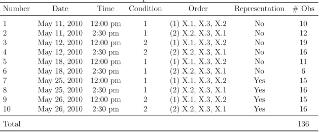
percentages at the top of each decision sheet. The stapling was done such that subjects would be forced to hold the representation of Option A in order to make the first few decisions. Though I imagined that this nuance might influence the degree of attachment to Option A, it had virtually no effect.14 A total of 136 subjects participated in the study across 10 experimental sessions. Table 1 provides the dates, times, orders and details of all sessions.
Table 1: Experimental Sessions
Number Date Time Condition Order Representation # Obs
1 May 11, 2010 12:00 pm 1 (1) X.1, X.3, X.2 No 10
2 May 11, 2010 2:30 pm 1 (2) X.2, X.3, X.1 No 12
3 May 12, 2010 12:00 pm 2 (1) X.1, X.3, X.2 No 19
4 May 12, 2010 2:30 pm 2 (2) X.2, X.3, X.1 No 16
5 May 18, 2010 12:00 pm 1 (1) X.1, X.3, X.2 No 11
6 May 18, 2010 2:30 pm 1 (2) X.2, X.3, X.1 No 6
7 May 25, 2010 12:00 pm 1 (1) X.1, X.3, X.2 Yes 15
8 May 25, 2010 2:30 pm 1 (2) X.2, X.3, X.1 Yes 16
9 May 26, 2010 12:00 pm 2 (1) X.1, X.3, X.2 Yes 15
10 May 26, 2010 2:30 pm 2 (2) X.2, X.3, X.1 Yes 16
Total 136
Notes: ‘Representation’ refers to whether or not Option A was physically represented by stapling
miniature bills or bills and percentages to the decision sheet.
In order to provide incentive for truthful revelation of preferences, subjects were randomly paid for one of their choices.15 The instructions fully described the payment procedure and the mechanism for carrying out randomization of payments, two ten-sided die. The randomization was described in independent terms. That is, mention was made of rolling die first for Option A and then for Option B and an example was given. Subjects earned, on average, $23 from the study including a $5 minimum payment that was added to all experimental earnings.
14Andreoni and Sprenger (2010) use uncertainty equivalents to test expected utility and investigate
violations of first order stochastic dominance near to certainty. In the non-representation treatments for Condition 1.3 the findings are reproduced. However, in the representation treatments for Condition 1.3, stochastic dominance violations at certainty are reduced to zero. See Sections 4.2 and 4.3 for discussion.
15This randomization device introduces a compound lottery to the decision environment as each
individual made around 440 choices over their 22 tasks. Reduction of compound lotteries does not change the general equivalence predictions for standard expected utility, prospect theory and dis-appointment aversion discussed above. However, to the extent that the compound lottery changes perceived referents, the randomization introduces complications into the KR analysis as it creates a potential link between choices and referents across tasks. See Section 4.1 for further discussion.
4
Results
The results are presented in three sub-sections. The first sub-section provides a brief summary of the elicited risk attitudes across the two conditions and non-parametric tests demonstrating risk aversion in the probability equivalent tasks and virtual risk neutrality in the certainty equivalent tasks. Second, motivated by these non-parametric results, the KR utility model is estimated and compelling out-of-sample predictions for uncertainty equivalent tasks at both the aggregate and individual level are provided. The third sub-section is devoted to discussing within-subjects results with data from Andreoni and Sprenger (2010), which also demonstrate significant differences in elicited risk preferences between certainty and probability equivalent techniques.
4.1
Risk Attitudes
Of the 136 individuals who participated in the primary experiment, 70 individuals participated in Condition 1 and 66 participated in Condition 2. As in most price-list style experiments, a number of subjects switch from Option A to Option B and then back to Option A.16 Three subjects (4.3%) in Condition 1 and eleven subjects (16.7%) in Condition 2 featured multiple switch points in at least one task. The majority of multiple switching occurred in Condition 2.3, indicating that this task may have been confusing to subjects.17 Attention is given to the 122 subjects who had unique switch points in all 22 decision tasks.18 This results in 1474 individual decisions in Condition 1 and 1210 decisions in Condition 2. Of these 2684 total decision tasks, in a small percentage (0.60%) the subject preferred Option A for all rows and in a larger percentage (4.14%) the subject preferred Option B for all rows. These responses provide only one-sided bounds on the interval of the subject’s response. The other bound is imputed via top and bottom-coding accordingly.19
16Around 10 percent of subjects feature multiple switch points in similar price-list experiments (Holt
and Laury, 2002; Meier and Sprenger, 2010), and as many as 50 percent in some cases (Jacobson and Petrie, 2009). Because such multiple switch points are difficult to rationalize and may indicate subject confusion, researchers often exclude such observations or mechanically enforce single switch points. See Harrison, Lau, Rutstrom and Williams (2005) for discussion.
17Five of 11 multiple switchers in Condition 2, had multiple switching in only Condition 2.3, one
had multiple switching in Conditions 2.1 and 2.3, two had multiple switching in Conditions 2.2 and 2.3, and three had multiple switching in all three subconditions.
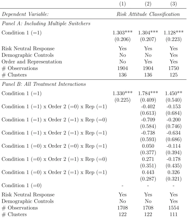
18All results are maintained when including multiple switchers and taking their first switch point
as their choice. See Appendix Table A1 for details.
19For example if an individual chose Option A at all rows in a probability equivalent including when
Option B was a 100% chance of getting $30, I topcode the interval as [100,100]. Virtually all of the
bottom-coded responses, 100 of 111, were decisions in Condition 2.3 where the bottom-coded choice would be preferring $10 with certainty to a given gamble over $0 and $30. No bottom-coded responses
A variety of demographic, cognitive and attitudinal data were collected after the study was concluded in order to provide a simple balancing test. Table 2 compares data across experimental conditions for survey respondents.20 Though some differences do exist, particularly in academic year, subjects were broadly balanced on observable characteristics, simple numeracy and cognitive ability scores, and subjectively reported risk attitudes.21 An omnibus test from the logit regression of condition assignment on all survey variables for 111 of 122 individuals with complete survey data does not reject the null hypothesis of equal demographic, cognitive and attitudinal character-istics across conditions (χ2 = 14.1, p = 0.12). Because the randomization is at the session level, this helps to ensure that accidental selection issues are not driving the experimental results. Additional within-subjects results unaffected by selection are provided in Sub-Section 4.3, along with demonstrations of robustness to controlling for demographic differences.
I begin by investigating behavior in Conditions 1.1, 1.2, 2.1 and 2.2. With the excep-tion of the KR preference model, all discussed theories predict experimental equivalence across these conditions. That is, elicited risk attitudes should be identical whether one asks the probability equivalent of a given certain amount or the certainty equivalent of a given gamble. Figure 4 presents median data for the 122 individuals with unique switch points along with a dashed black line corresponding to risk neutrality. The ex-perimentally controlled parameter is presented on the horizontal axis and the median subject response is presented on the vertical axis.
Apparent from the median data is the systematic difference in elicited risk attitudes between certainty and probability equivalents. When fixing a stochastic gamble and trading for increasing certain amounts in Conditions 2.1 and 2.2, subjects display virtual risk neutrality. When fixing a certain amount and trading for increasing gambles in Conditions 1.1 and 1.2 subjects display risk aversion.
For each experimental task, decisions are classified as being risk neutral, risk averse or risk loving. These classifications recognize the interval nature of the data. For
arose in Condition 1 or 2.1 where the lowest Option B outcome was $0 with certainty.
20111 of 122 subjects completed all survey elements. 60 of 67 subjects in Condition 1 and 51 of 55
subjects in Condition 2 provided complete survey responses. Non-response is unrelated to condition as Condition 1 accounts for 54-55 percent of the data in both the respondent and full samples.
21Numeracy is measured with a six question exam related to simple math skills such as division
and compound interest previously validated in a number of large and representative samples (Lusardi and Mitchell, 2007; Banks and Oldfield, 2007; Gerardi, Goette and Meier, 2010). Cognitive ability is measured with the three question Cognitive Reflection Test introduced and validated in Frederick (2005). Subjective risk attitudes are measured on a 7 point scale with the question,“How willing are you to take risks in general on a scale from 1 (unwilling) to 7 (fullly prepared)” previously validated in a large representative sample (Dohmen, Falk, Huffman, Sunde, Schupp and Wagner, 2005).
Table 2: Summary Statistics and Balancing Test
Total Condition 1 Condition 2
N = 122 N = 67 N = 55
Variable # Obs Mean Mean Mean t-statistic p-value
(s.d) (s.d) (s.d.)
Male (=1) 119 0.46 0.42 0.52 1.12 (p=0.27)
(0.50) (0.50) (0.50)
Academic Year 122 2.63 2.45 2.85 2.10 (p=0.04)
(1.08) (1.05) (1.08)
Grade Point Average 120 3.20 3.25 3.15 -1.26 (p=0.21)
(.42) (.44) (.39)
English 1stLanguage (=1) 122 0.56 0.51 0.62 1.22 (p=0.22)
(0.50) (0.50) (0.49)
Smoker (=1) 122 0.04 0.03 0.05 0.68 (p=0.50)
(0.20) (0.17) (0.23)
Weekly Spending ($) 122 89.68 85.00 95.38 0.64 (p=0.53)
(89.49) (68.63) (110.12)
Risk Attitudes (1-7) 122 3.84 3.70 4.00 1.39 (p=0.17)
(1.19) (1.22) (1.14)
Cognitive Ability Score (1-3) 117 1.79 1.86 1.70 -0.83 (p=0.41)
(1.05) (1.08) (1.01)
Numeracy Score (1-6) 120 5.75 5.78 5.71 -0.76 (p=0.45)
(0.54) (0.52) (0.57)
Omnibusχ2 = 14.1, (p= 0.12)
Notes: Summary statistics for 122 subjects with unique switch points in all 22 decision tasks. # Obs
refers to the number of responses to each question. Omnibusχ2test statistic corresponding to the null
hypothesis of zero slopes in logit regression with 111 subjects with complete survey data of condition assignment on all survey variables with robust standard errors.
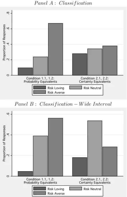
example, a decision is coded as risk neutral if the risk neutral response lies in the interval generated by the subject’s switch point. Figure 5, Panel A presents these classifications. Whereas the distributions of risk averse, neutral and loving responses are somewhat even in the certainty equivalents of Condition 2, the majority of responses are risk averse in the probability equivalents of Condition 1. Proportionately nearly twice as many responses are classified as risk averse in probability equivalents relative to certainty equivalents. As this may be a strict classification of responses, Figure 5, Panel B extends the interval of the switch point to +/− one choice. By this wider
interval measure the majority of the data in Condition 1 remains risk averse, while the majority of the data in Condition 2 is now classified as risk neutral.
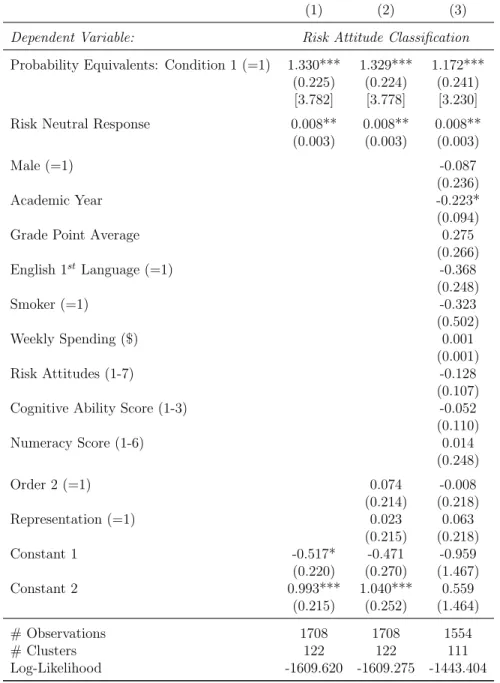
Table 3 presents ordered logit regressions for the classification of responses of Figure 5, Panel A with standard errors clustered on the individual level. The dependent
Figure 4: Conditions 1.1, 1.2, 2.1, and 2.2 Responses Risk Neutral Risk Neutral Risk Neutral Risk Averse Risk Averse Risk Averse Risk Loving Risk Loving Risk Loving 0 0 0 20 20 20 40 40 40 60 60 60 80 80 80 100 100 100 PE (p;30,0) PE (p;30,0) PE (p;30,0) 0 0 0 20 20 20 40 40 40 60 60 60 80 80 80 100 100 100
Given Certain Amount / 30
Given Certain Amount / 30 Given Certain Amount / 30
Certain Referent Certain Referent Certain Referent Condition 1.1 Condition 1.1 Condition 1.1 0 0 0 20 20 20 40 40 40 60 60 60 80 80 80 100 100 100 PE (p;30,10) PE (p;30,10) PE (p;30,10) 0 0 0 20 20 20 40 40 40 60 60 60 80 80 80 100 100 100
Given Certain Amount / 30
Given Certain Amount / 30 Given Certain Amount / 30
Certain Referent Certain Referent Certain Referent Condition 1.2 Condition 1.2 Condition 1.2 Risk Loving Risk Loving Risk Loving Risk Averse Risk Averse Risk Averse Risk Neutral Risk Neutral Risk Neutral 0 0 0 20 20 20 40 40 40 60 60 60 80 80 80 100 100 100 CE/30 CE/30 CE/30 0 0 0 20 20 20 40 40 40 60 60 60 80 80 80 100 100 100
Given Gamble (p;30,0)
Given Gamble (p;30,0) Given Gamble (p;30,0)
Stochastic Referent Stochastic Referent Stochastic Referent Condition 2.1 Condition 2.1 Condition 2.1 0 0 0 20 20 20 40 40 40 60 60 60 80 80 80 100 100 100 CE/30 CE/30 CE/30 0 0 0 20 20 20 40 40 40 60 60 60 80 80 80 100 100 100
Given Gamble (p;30,10)
Given Gamble (p;30,10) Given Gamble (p;30,10)
Stochastic Referent Stochastic Referent Stochastic Referent Condition 2.2 Condition 2.2 Condition 2.2 Median Response Median Response Median Response 25-75 %-ile 25-75 %-ile 25-75 %-ile 5-95 %-ile 5-95 %-ile 5-95 %-ile Model Fit Model Fit Model Fit
Note: Median data from 122 experimental subjects with unique switching points in all 22 decision tasks. Dashed black line corresponds to risk neutrality. Solid red line for Conditions 1.1 and 1.2 corresponds to KR model fit with ˆλ = 3.4. The KR model predicts risk aversion for probability equivalents in Conditions 1.1 and 1.2 and risk neutrality for certainty equivalents in Conditions 2.1 and 2.2.
variable isRisk Attitude, which takes the value -1 for a risk loving classification, 0 for risk neutrality, and +1 for a risk averse response. The natural order of Risk Attitude corresponds to increasing risk aversion. These regressions control for condition and the variableRisk Neutral Response. Risk Neutral Response is coded from 0 to 100 and expresses in percentage terms the dashed line of risk neutrality in Figure 4. That is,Risk Neutral Responseis either the given certain amount’s risk neutral probability equivalent (in Condition 1), or the given gamble’s expected value divided by 30 (in Condition 2). This helps to control for experimental variation that might be related to elicited risk attitudes under non-EU preference models such as non-linear probability weighting. Certain specifications additionally control for order and representation effects as well as the collected demographic and attitudinal characteristics for individuals who responded
Figure 5: Conditions 1.1, 1.2, 2.1, and 2.2 Classifications P anel A: Classif ication
0
0
0 .2
.2
.2 .4
.4
.4 .6
.6
.6 .8
.8
.8
Proportion of Responses
Proportion of Responses
Proportion of Responses Condition 1.1, 1.2:
Condition 1.1, 1.2: Condition 1.1, 1.2:
Probability Equivalents
Probability Equivalents Probability Equivalents
Condition 2.1, 2.2:
Condition 2.1, 2.2: Condition 2.1, 2.2:
Certainty Equivalents
Certainty Equivalents Certainty Equivalents
Risk Loving
Risk Loving Risk Loving
Risk Neutral
Risk Neutral Risk Neutral
Risk Averse
Risk Averse Risk Averse
P anel B : Classif ication−W ide Interval
0
0
0 .2
.2
.2 .4
.4
.4 .6
.6
.6
Proportion of Responses
Proportion of Responses
Proportion of Responses Condition 1.1, 1.2:
Condition 1.1, 1.2: Condition 1.1, 1.2:
Probability Equivalents
Probability Equivalents Probability Equivalents
Condition 2.1, 2.2:
Condition 2.1, 2.2: Condition 2.1, 2.2:
Certainty Equivalents
Certainty Equivalents Certainty Equivalents
Risk Loving
Risk Loving Risk Loving
Risk Neutral
Risk Neutral Risk Neutral
Risk Averse
Risk Averse Risk Averse
Note: The figure presents classifications of responses from 122 experimental subjects with unique switching points in all 22 decision tasks. The KR model predicts risk aversion for probability equivalents in Conditions 1.1 and 1.2 and risk neutrality for certainty equivalents in Conditions 2.1 and 2.2. Panel A provides the classifications based on the interval of a subject’s switch point. Panel B provides classifications based on a wider interval of the switch point +/−one choice.
in full to the post-study survey. Across specifications, subjects in Condition 1 are significantly more likely to have risk averse responses. Odds ratios for being classified as risk averse relative to risk neutral or risk loving are provided in brackets. Subjects randomly assigned to Condition 1 are between three and four times more likely to exhibit risk aversion than those assigned to Condition 2.22
These simple tests indicate an endowment effect for risk. In certainty equivalents tasks, subjects are generally risk neutral. In probability equivalents tasks, subjects are generally risk averse. Standard expected utility, prospect theory and disappointment aversion all predict experimental equivalence across these two environments. The data are potentially consistent with the KR model, with its possibility of a stochastic ref-erence distribution. However, the obtained data are not directly consistent with the refined PPE concept, which would also predict identical behavior across conditions.
In applying the equilibrium concepts from KR, I consider some form of narrow bracketing within a given row of a choice task. That is, the subject considers a choice in a given row between Option A, representing some fixed amount or gam-ble, G, and Option B, representing some fixed amount or gamble, F. As discussed in Section 2.1.3, choosing Option A over Option B therefore implies the PPE rela-tion U(G|G) > U(F|F). However in the KR model there is some ambiguity in the bracketing of the referent. It is possible, for instance, to consider the referent to be the distribution induced by all choices in the task, or even all choices in the entire experiment. Such a specification could potentially revive PPE as a viable organization of the data. However solving for a PPE in these cases is computationally intensive and a somewhat implausible calculation on the part of subjects. The narrow bracketing used in this analysis is a direct application of the KR equilibrium in choices between lotteries.
Equilibrium behavior even in its simplest form may be a stringent requirement for experimental subjects. A body of evidence from strategic environments argues against equilibrium logic in the laboratory (Camerer et al., 2004; Costa-Gomes and Craw-ford, 2006; Crawford and Iriberri, 2007; Costa-Gomes et al., 2009). Resulting process models such as level-k thinking are argued to be organized around initial reactions to experimental environments. Koszegi and Rabin (2006) provide a similar indication, suggesting that referents are established as probabilistic beliefs held at the moment an individual first focused on a decision. In our environment, subjects may first focus their thinking on the fixed element in a given series of decisions. If so, then the referent may
22Results are maintained with the inclusion of multiple switchers. Additionally, no interactions for
Table 3: Probability and Certainty Equivalent Risk Attitude Regressions
(1) (2) (3)
Dependent Variable: Risk Attitude Classification
Probability Equivalents: Condition 1 (=1) 1.330*** 1.329*** 1.172***
(0.225) (0.224) (0.241)
[3.782] [3.778] [3.230]
Risk Neutral Response 0.008** 0.008** 0.008**
(0.003) (0.003) (0.003)
Male (=1) -0.087
(0.236)
Academic Year -0.223*
(0.094)
Grade Point Average 0.275
(0.266)
English 1st Language (=1) -0.368
(0.248)
Smoker (=1) -0.323
(0.502)
Weekly Spending ($) 0.001
(0.001)
Risk Attitudes (1-7) -0.128
(0.107)
Cognitive Ability Score (1-3) -0.052
(0.110)
Numeracy Score (1-6) 0.014
(0.248)
Order 2 (=1) 0.074 -0.008
(0.214) (0.218)
Representation (=1) 0.023 0.063
(0.215) (0.218)
Constant 1 -0.517* -0.471 -0.959
(0.220) (0.270) (1.467)
Constant 2 0.993*** 1.040*** 0.559
(0.215) (0.252) (1.464)
# Observations 1708 1708 1554
# Clusters 122 122 111
Log-Likelihood -1609.620 -1609.275 -1443.404
Notes: Coefficients from ordered logit of Risk Attitude classification on control variables, measured
from probability and certainty equivalents of Conditions 1.1, 1.2, 2.1, and 2.2. Risk Attitudetakes the
value -1 for risk loving, 0 for risk neutral, and +1 for risk averse. Standard errors clustered on the individual level in parentheses. Odds ratios for Condition 1 in brackets, calculated as the exponentiated coefficient. Column (3) features data from 111 subjects who also completed the post-study survey.
Level of significance: *p <0.1, **p <0.05, ***p <0.01
sensibly change across the conditions of our experiment. In certainty equivalents the referent will be stochastic, while in probability equivalents the referent will be certain. See Section 5 for further discussion.
4.2
Estimating KR Preferences
Under the assumption that subjects organize their thinking around the fixed element in a series of decisions, the KR model with exogenously manipulated referents rationalizes the data. Importantly, such a model is easily implemented econometrically. The KR model motivated above is described by one key parameter,λ, the degree of loss aversion, which can be estimated at either the group or individual level via non-linear least squares.
Using the data from probability equivalent Conditions 1.1 and 1.2, the midpoint of the interval implied by a subject’s switch point is taken as the valueq∗ in equation (2). Equation (2) is then estimated via non-linear least squares with standard errors clus-tered on the subject level. The aggregate estimate is ˆλ= 3.41 (s.e.= 0.34). The null hypothesis of zero loss aversion,λ = 1, is rejectedF1,66= 49.06, p <0.01. This value of loss aversion is consistent with loss aversion estimates from other contexts (Tversky and Kahneman, 1992; Gill and Prowse, 2010; Pope and Schweitzer, Forthcoming) and is closely in line with the often discussed benchmark of losses being felt twice as severely as gains, λ= 3, η = 1 (Koszegi and Rabin, 2006, 2007).23 Figure 4 presents predicted values from this aggregate regression as the solid red line for Conditions 1.1 and 1.2. The aggregate data matches well the fitted model’s predicted hump-shaped deviation from risk neutrality. Of course, the KR preference model predicts risk neutrality in Conditions 2.1 and 2.2.
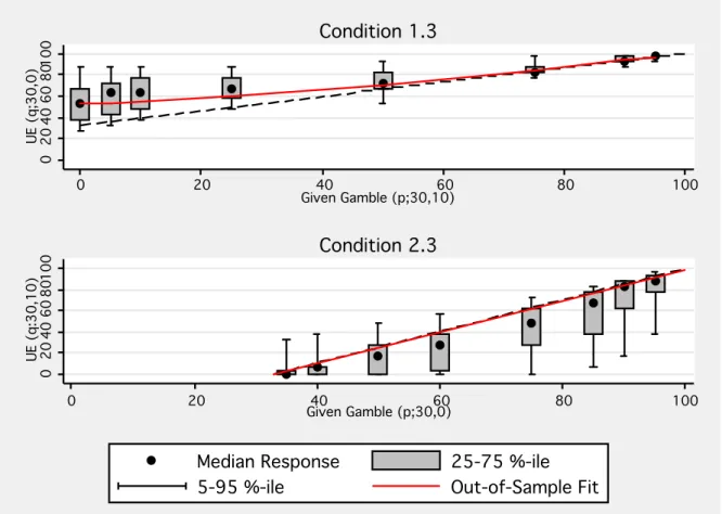
In order to evaluate the predictive validity of the KR preference model, it can be tested out of sample with alternative segments of the data. As noted above, the KR preference model with a stochastic referent predicts risk neutrality in Condition 2.3 and predicts a particular shape of quadratically declining risk aversion in Condition 1.3. Figure 6 presents data from these conditions as well as out-of-sample predictions for KR model with the estimated ˆλ= 3.4. Though the KR prediction of risk neutrality breaks down at the intermediate probabilities of Condition 2.3, in Condition 1.3, the out-of-sample prediction closely matches aggregate behavior.24
23The functional form of Tversky and Kahneman (1992) does not feature consumption utility and
so the loss aversion estimate of ˆλ= 2.25 in their paper is a direct measure of losses being felt twice
as severely as gains.
24Additionally, Condition 1.3 reproduces the general shape and level of the uncertainty equivalents
discussed in Andreoni and Sprenger (2010) demonstrating a slightly convex relationship between given gambles and their uncertainty equivalents. However, Andreoni and Sprenger (2010) document the convexity becoming sharper as the given gamble approaches certainty, and this result is not present in the data. Minor differences in experimental detail may account for the difference atp= 0
between the present results and Andreoni and Sprenger (2010) including a different number and order of tasks and slightly changed tasks. The Andreoni and Sprenger (2010) price lists were designed with decision aids of checked top and bottom rows. The task used in Condition 1.3 was not. More
Figure 6: Conditions 1.3 and 2.3 0
0
0 20
20
20 40
40
40 60
60
60 80
80
80 100
100
100 UE (q;30,0)
UE (q;30,0)
UE (q;30,0) 0
0 0
20
20 20
40
40 40
60
60 60
80
80 80
100
100 100
Given Gamble (p;30,10)
Given Gamble (p;30,10) Given Gamble (p;30,10)
Condition 1.3
Condition 1.3 Condition 1.3
0
0
0 20
20
20 40
40
40 60
60
60 80
80
80 100
100
100
UE (q:30,10)
UE (q:30,10)
UE (q:30,10) 0
0 0
20
20 20
40
40 40
60
60 60
80
80 80
100
100 100
Given Gamble (p;30,0)
Given Gamble (p;30,0) Given Gamble (p;30,0)
Condition 2.3
Condition 2.3 Condition 2.3
Median Response
Median Response Median Response
25-75 %-ile
25-75 %-ile 25-75 %-ile
5-95 %-ile
5-95 %-ile 5-95 %-ile
Out-of-Sample Fit
Out-of-Sample Fit Out-of-Sample Fit
Note: Median data from 122 experimental subjects with unique switching points in all 22 decision tasks. Dashed black line corresponds to risk neutrality. Solid red lines correspond to out-of-sample KR model prediction with ˆλ = 3.4 as estimated in Conditions 1.1 and 1.2.
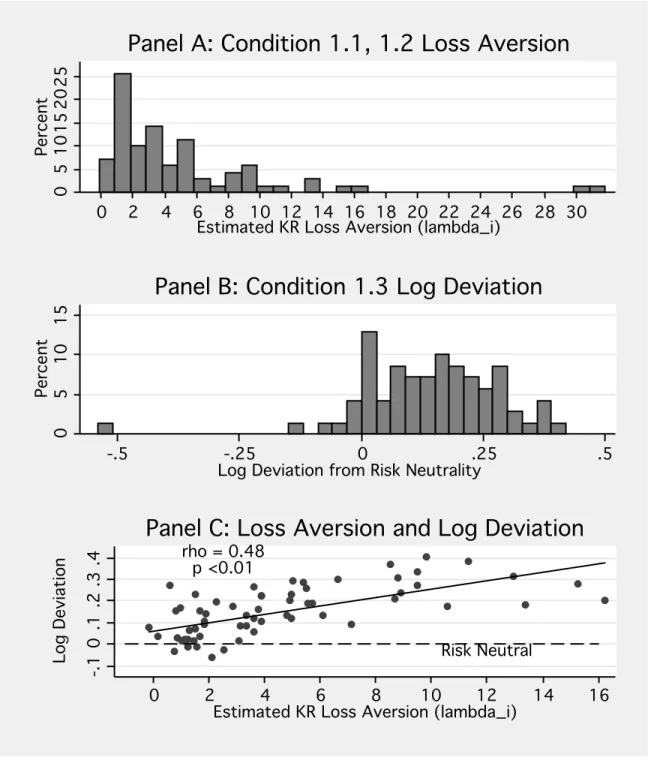
In addition to aggregate out-of-sample predictions, for the 67 subjects in Condition 1, individual analyses can be conducted. Using the data from Conditions 1.1 and 1.2, the degree of loss aversion,λi, can be estimated following equation (2). These individual
estimates, ˆλi, can be correlated with behavior in Condition 1.3. As discussed in Section
3.1, the deviation from risk neutrality is predicted to increase withλi.
importantly, however, appears to be the presence of the physical representation of Option A. The sharpened convexity atp= 0 in Andreoni and Sprenger (2010) is driven by individuals who violate
first order stochastic dominance close to certainty. They document individual dominance violation rates betweenp= 0 and p= 0.05 of around 17.5 percent across three tasks. When Option A is not
physically represented, a similar violation rate of 13.5 percent is found. However, when Option A is physically represented, zero violations of stochastic dominance at certainty are observed. The effect of physical representation on the proportion of individuals violating stochastic dominance at certainty is significant (z= 2.09, p <0.05).