Munich Personal RePEc Archive
Nonlinear exchange rate pass-through in
timber products: the case of oriented
strand board in Canada and the United
States
Goodwin, Barry K. and Holt, Matthew T. and Prestemon,
Jeffrey P.
University of Alabama, North Carolina State University, USDA
Forest Service
22 August 2012
Nonlinear Exchange Rate Pass–Through in Timber Products: The
Case of Oriented Strand Board in Canada and the United States
Barry K. Goodwin∗
Department of Agricultural and Resource Economics North Carolina State University
Matthew T. Holt†
Department of Economics, Finance, and Legal Studies
University of Alabama
Jeffrey P. Prestemon‡
USDA Forest Service
Southern Research Station
This Draft: August 22, 2012
Abstract
We assess exchange rate pass–through (ERPT) for U.S. and Canadian prices for oriented strand board (OSB), a wood panel product used extensively in U.S. residential construction. Because of its prominence in construction and international trade, OSB markets are likely sensitive to general economic conditions. In keeping with recent research (e.g., Al-Abri and Goodwin, 2009; Larue et al., 2010), we examine regime– specific ERPT effects; we use a smooth transition vector error correction model. We also build on work by Nogueira, Jr. and Le´on-Ledesma (2011) and Chew et al. (2011) in considering ERPT asymmetries associated with a measure of general macroeconomic activity. Our results indicate that during expansionary periods ERPT is modest, at least initially, but during the recent financial crises ERPT effects were quite large.
Keywords: Exchange rate pass–through, oriented strand board, smooth transition model, unemployment
JEL Classification Codes: E32, F10; F30; F41; L16
∗Department of Agricultural and Resource Economics and Department of Economics, North Carolina State
Uni-versity, Campus Box 8109, Raleigh, NC 27695–8109, USA. Telephone: 919-515-4620. Fax: 765-515-1824. E-mail: barry [email protected].
†
Corresponding Author: Department of Economics, Finance, and Legal Studies, University of Alabama, Box 870224, Tuscaloosa, AL 35487-0224, USA. Telephone: 205-348-8980. Fax: 205-348-0590. E-mail: [email protected].
‡Forestry Sciences Laboratory, P.O. Box 12254, 3041 Cornwallis Road, Research Triangle Park, NC, 27709-2254,
1 Introduction
Questions regarding the extent of exchange rate pass–through (ERPT) into import prices, in other
words, the degree to which exchange rate shocks evoke equilibrating price response for traded
com-modities and goods, have long been of interest to economists and policy makers. Much of the recent
interest in this topic can perhaps be traced to the observation that estimated ERPT effects are
gen-erally reported to be small (Goldberg and Knetter, 1997) For example, a widely cited rate of pass–
through into aggregate import price is approximately 50%, as reported by Goldberg and Knetter
(1997). In addition to relatively low rates of ERPT, there is also mounting evidence that they
have been declining over time; see, for example, Bailliu and Fujii (2004), Campa and Goldberg
(2005), and Marazzi and Sheets (2007), among others. Correspondingly, several strands of the
ERPT literature have evolved. One is the so called macro strand, where the focus is on
deter-mining the extent of ERPT to import prices at the aggregate level and, secondarily, the extent to
which such responses are passed along to consumers (see, e.g., Gagnon and Ihrig, 2004). Another
strand focuses on determining the extent to which ERPT impacts import prices at the industry or
commodity level, where incomplete pass–through is often conjectured to be a function of the market
structure of the industry being examined. Examples of work in this vain include Knetter (1989)
and Pollard and Coughlin (2004). Of interest is that empirical estimates of long–run ERPT at the
industry or commodity level are often even smaller than those obtained by using more aggregated
data.
Over the years various theories and/or methodological refinements have been explored in an
at-tempt to account for low and/or declining rates of ERPT. Of interest is that a small number of recent
studies have examined the possibility that there are asymmetries or nonlinearities in pass–through,
that is, for example, that a currency depreciation could have different impacts on import prices than
would an appreciation or, similarly, that large changed may have different effects than small ones.
In one of the earliest studies of this sort, Mann (1986) found evidence of asymmetric pass–through
effects. Likewise, by employing aggregate data for seven Asian Pacific countries, Webber (2000)
re-ports substantial evidence of asymmetric pass–through effects for five of these. Bussiere (2007)
con-siders pass–through into import and export prices in G7 countries, and finds substantial evidence of
corresponding nonlinear models of pass through. Karoro, Aziakpono and Cattaneo (2009) consider
asymmetries in pass–through to import prices in South Africa; they find evidence that ERPT is
higher during periods of rapid appreciation relative to deprecation. As well, Al-Abri and Goodwin
(2009) update the data used by Campa and Goldberg (2005) and also allow for threshold effects
with respect to ERPT into G7 country import prices. Overall, they find substantial evidence of
non-linearities in pass–through effects. In a closely related study, Larue, Gervais and Rancourt (2010)
examine the possibility asymmetric ERPT into export prices for pork meat from Canada to Japan
and the U.S. by using threshold cointegration techniques.
Many of the studies outlined above have focused on estimating pass–through effects by using
either import prices at either the aggregate level or for specific industries. Comparatively few
stud-ies have focused on pass–through effects at the individual commodity level. In part this is because
commodities are typically homogeneous and to be traded in something close to perfectly
competi-tive market conditions. The implication is that the ability of exporting firms to exert any market
power over pricing combined with the perfect arbitrage conditions of the “law of one price” (LOP)
are thought to result in complete ERPT for commodity import prices. In short, commodities are
thought to have flexible or flex import prices. Even so, there is evidence that, at least in some
instances, there is incomplete pass–through for commodities. Jabara and Schwartz (1987) explore
ERPT for Japanese import prices for five agricultural commodities, and find evidence of
incom-plete pass–through as well as evidence of asymmetric responses to exchange rate shocks for several
commodities. As well, they find substantial evidence of asymmetric responses to exchange rates for
several commodities. Likewise, Uusivuori and Buongiorno (1991) examine ERPT for a number of
U.S. forest product exports to Europe and Japan, and find both that pass–through is incomplete
and that its effects are asymmetric depending on whether the exchange rate is appreciating or
de-preciating. Finally, Parsley (1995) examines ERPT for five specific products exported from Japan
to the United States. In this study asymmetry in (real) exchange rate effects were also allowed for;
the results show there is are apparent declines in ERPT during periods of dollar appreciation.
In general ERPT is an important indicator of the operation and performance of markets for
internationally–traded commodities such as OSB. A lack of pass–through may reflect imperfect
arbitrage, inefficient trade, inflexible prices (perhaps due to contracts or menu pricing practices),
pass–through indicates that standard arbitrage behavior, which is often assumed to hold in absolute
terms in conceptual and empirical models of trade, may in fact not be supported empirically. In
any event, attaining deeper insights into the nature of ERPT at the primary commodity level is an
important agenda in the modern empirical trade literature; there is scope for further work.
To begin, it is surprising that comparatively few studies have explored ERPT at the product or
commodity level. As well, while there is mounting evidence that asymmetries or, more generally,
nonlinearities are a feature of the exchange rate effect on import prices, it is also surprising that
comparatively few studies have examined these effects by using modern time series methods, and
especially so when ERPT is examined at the commodity level.1 The overall goals of this paper
are then: (1) to examine ERPT in import prices for a highly traded, homogeneous commodity;
and (2) to examine in a general testing and estimation framework the role of nonlinearities in
ERPT. Specifically, we examine the (potentially nonlinear) impacts of exchange rates on U.S.
import prices and Canadian export prices for oriented strand board (OSB). Oriented strand board
represents an interesting case study for which to examine ERPT at the product level. It is a
homogeneous product that is widely used in residential and commercial construction throughout
North America. As illustrated in Figure 1, in recent years the U.S. has produced more OSB
than Canada, but Canada exports both a far higher amount as well as a greater percentage of its
total production than does the United States (on average 84% versus 1.6%). Moreover, as also
illustrated in Figure 1 the overwhelming majority of all Canadian OSB exports are destined for
the United States. While prior work has examined pass–through issues for international trade
in various timber products (see, e.g., Uusivuori and Buongiorno, 1991; Bolkesjø and Buongiorno,
2006), to our knowledge similar questions have not been addressed for panel products manufactured
wood products. Taken together the evidence suggests that additional insights into ERPT at the
product level can be attained by conducting a careful analysis of U.S. and Canadian OSB price
relationships.
1
2 Conceptual Framework
There is a vast literature that examines questions regarding the law of one price in the context
of international (regional) price behavior; see, for example, Goodwin, Holt and Prestemon (2011)
along with references therein for a recent review of this research. The micro–foundations underlying
exchange rate pass–through are identical to those that motivate the LOP; however, investigations
of ERPT highlight the separate effects of price and exchange rate shocks in commodities that are
traded across markets with different currencies. In that it is common for internationally–traded
commodities to be invoiced in a common currency across different national markets (e.g., the U.S.
dollar or the Euro), exchange rates may still have an impact on price linkages if the internal markets
being considered have different currencies.
Following Goldberg and Knetter (1997), in the classical pass–through literature the basic long–
run price relationship may be stated as:
Pit = Eβ
1 t P
β2
xt, β1, β2>0, t= 1, . . . , T, (1)
wherePitis the (nominal) import price in countryifor the good in question in periodt(denominated
in countryi’s currency);Pxtis the corresponding (nominal) export price in countryj(denominated
in countryj’s currency); andEtis the nominal exchange rate, expressed in terms of the importer’s
currency (i.e., countryi’s) relative to the exporter’s currency (i.e., countryj’s). As well,β1 and β2
are parameters such that with perfect pass–through β1 =β2 = 1. It is natural to convert (1) to
natural logarithmic form, so that the price relationship may be written as:
pit = β1et+β2pxt, (2)
where lower case letters denote variables expressed in natural log form. If (2) is estimated as is (and
for the moment ignoring any possible time series complications associated with the data), then a
model for testing the impact of exchange rates on import prices could be specified simply as:
where β1 and β2 are parameters to be estimated and εt is an additive error term such that εt ∼
iid(0, σ2). In this case a test of full (complete) exchange rate pass–through would be associated
with a test of the hypothesis H0 :β1 =β2 = 1.
The specification defined by (1)–(3) assumes pxt is measured in the exporter’s currency. In the
case where exports are invoiced in the importer’s currency, the exporter’s price may be written as
Pxt = ˜Pxt/Et, where ˜Pxt is the export price expressed in the importing country’s currency. In this
later case, that is, when prices are invoiced in the importer’s currency, the model in (3) may be
rewritten as:
pit = (β1−β2)et+β2p˜xt+εt. (4)
For complete pass–through we again requireβ1=β2= 1, which in turn reduces (4) to a stochastic
version of the law–of–one–price relationship. In other words, with common currency pricing
com-plete pass–through implies that exchange rates should have no long–term (permanent) impact on
the import price.
Following recent literature (see, e.g., Campa, Goldberg and Gonzalez-Minguez, 2005), we could
further modify the model to allow for the possibility that exporting firms, presumably operating
in an imperfectly competitive market environment, could maintain a fixed percentage markup over
their marginal cost. The assumption of imperfectly competitive market conditions seems relevant
for North American OSB markets. In 2006, a series of lawsuits were consolidated into a single
case in the U.S. District Court in Pennsylvania on behalf of aggrieved parties involved in OSB
purchases between June, 2002 and February, 2006. The suite alleged that the a number of major
North American OSB manufacturers, operating in both the United States and Canada, conspired
to maintain artificially high prices for OSB during the June, 2002 through February, 2006 period.2
In any case, to modify the model to allow for imperfectly competitive behavior, we can rewrite ˜px,t
as:
˜
pxt = mkupxt(et) +mcxt, (5)
where mkupxt(et) denotes the percentage markup and mcxt denotes marginal cost, both in
loga-rithmic form. As well, and as indicated by the notation in (5), the markup may also vary with the
2
exchange rate. Again, following Campa, Goldberg and Gonzalez-Minguez (2005), we may write the
markup in (5) as:
mkupxt(et) = φ+ Φet, (6)
whereφis a component of the markup that does not change with the exchange rate.
In the case were import prices are invoiced in importing firm’s currency (i.e., local currency
pricing), we may substitute (5) and (6) into (4) to obtain:
pit =α0+ (β1+β2(Φ−1))et+β2mcxt+εt, (7)
where α0 =φβ2. Several important observations may be drawn from (7). To begin, even if β1 =
β2 = 1 holds, incomplete pass–through may occur to the extent that exporting firms operate in an
imperfectly competitive market environment. Secondly, if (7) is viewed as a long–run relationship,
then we might still reasonably expect a non–zero intercept term to be present if, in fact, φ, the
constant mark–up parameter, is non–zero.3 In the literature there are many example of variants of
(7) being used to estimate ERPT effects. See, for example, Campa and Goldberg (2005).
The basic framework outlined above can be modified if there is reason to suspect that ERPT is
regime specific, that is, that the impact of exchange rates on rates on import prices varies with either
the magnitude or direction of adjustment of some other variable including but not limited to the
ex-change rate itself. To illustrate, as Al-Abri and Goodwin (2009) and Larue, Gervais and Rancourt
(2010) note, the markup equation in (6) might be such that the exchange rate response
parame-ter, Φ, varies depending on the size (or sign) of a change in exchange rates. For relatively small
exchange rate adjustments exporters may decide not to adjust the markup due to menu costs. But
for a large exchange rate adjustment, exporting firms may be forced to adjust markups in order to
maintain market share. Alternatively, under local currency pricing the exporting firm presumably
must still convert revenues earned in foreign currency into the home currency. Presumably doing
so involves transactions costs and, moreover, costs that might vary with the magnitude of recent
exchange rate movements.
3
In addition, α0 may also capture factors associated with the cost of trade if such factors are proportional to
In any event, the model in (7) can be modified in the following manner:
pit =α0+(β1+β2(Φ1(1−I{st>θ} )
+ Φ2I{st>θ}−1 ))
et+β2mcxt+εt, (8)
where θ is the threshold parameter, and where I{st>θ} is a Heaviside indicator function such that
I{st≤θ}= 1 ifst> θ and is 0 otherwise. Herestis the so called transition variable; it is the variable
that, in conjunction θ, determines the nature of nonlinear pass–through effects. Let st = f(zt),
where zt is some underlying variable and the form of the function f(.) is presumably known. For
example, and as already noted, zt might equalet−1, the (lagged) exchange rate, althoughzt could
be equated with other observed variables as well. Regarding the specification ofst in (8), it might
be that: (1)st=zt−k; or (2) thatst=zt−1−zt−2; or (3) thatst= (zt−1−zt−2)2. See, for example,
van Dijk, Ter¨asvirta and Franses (2002) for additional details. In any event, the important point
is that the markup varies depending on recent movements in zt, and therefore ERPT effects will
also vary with these changes.
As already noted, nonlinearities in ERPT effects could arise for reasons other than those
asso-ciated with exchange rate behavior. For example, in a recent study Chew, Ouliaris and Tan (2011)
considered import prices for Singapore, and allowed the ERPT effects into these prices to vary with
the business cycle.4 Their results confirmed there are asymmetric pass–through effects into
Singa-pore’s import price over the business cycle, with smaller pass–through occurring during expansions
as compared with retractions.
Business cycle effects with respect to ERPT in North American OSB markets might be
espe-cially relevant given that residential construction (a primary end–use for OSB) is quite sensitive to
economic downturns; indeed, housing starts are often asserted to be an important leading
indica-tor of overall economic activity (Leamer, 2007). As an empirical proposition then, it is certainly
plausible that markups and hence ERPT could vary with the business cycle even when considering
price response for a specific commodity such as OSB. In terms of (8), the idea would be to linkzt
and hencestto one or more variables that transmit information regarding the stage of the business
cycle.
4
3 Data
3.1 Data Description
As indicated previously, we focus on prices for oriented strand board (OSB) in Canada and the
United States. OSB is a manufactured wood product that was introduced in 1978, and is widely
used in residential and commercial construction, with the bulk of OSB produced in North America
originating in the Southern U.S. and Canada. For example, in 2009 and 2010 Canada and the
Southern U.S. produced nearly ninety–percent of all OSB otherwise produced in North America
(Engineered Wood Product Association, 2010). OSB is constructed by using waterproof and heat
cured resins and waxes, and consists of rectangular shaped wood strands that are arranged in
oriented layers. As well, it is manufactured in long, continuous mats which are then cut into panels
of varying sizes. As a panel product OSB is similar to plywood, although it is generally considered
to have more consistency than plywood and is cheaper to produce. As indicated in Figure 1, the
Structural Board Association (SBA) reports that in 1980 OSB panel production in the U.S. was 135
million square feet (on a 3/8th’s inch basis) and in Canada was 616 million square feet. Comparable
numbers for 2010 were 10,838 million square feet produced in the U.S. and 4,700 million square
feet in Canada. The SBA also reports that by 2000 OSB production exceeded that of plywood,
and that by 2010 OSB production enjoyed a 58–percent market share among all panel products in
North America. Figure 1 illustrates the substantial growth in OSB production since 1995 as well
as the sharp decline in OSB production following the collapse of the U.S. housing market in 2007.
Considering the above, we focus on pass–through effects for OSB in two regional North
Amer-ican markets: (1) Eastern Canada (production deriving from plants in Ontario and Quebec); and
(2) the Southeast U.S. (production deriving from plants in Georgia, Alabama, Mississippi, South
Carolina, and Tennessee). The price data are for panels of 7/16th’s inch oriented strand board,
and are expressed in U.S. dollars per thousand square feet, that is, Canadian mills engage in local
currency pricing. All price data are observed on a weekly basis and were obtained from the
indus-try source Random Lengths.5 The regional OSB price data used are FOB mill price averages. The
5
period covered is from October 9, 1998 through August 20, 2010, the result being there are 620
usable weekly observations. A plot of the regional OSB price data converted to natural log form is
reported in Figure 2. In the analysis we propose treating the (natural logarithm) of the Southeast
U.S. as the effective import price (pi) and, following Wickremasinghe and Silvapulle (2004) and
Karoro, Aziakpono and Cattaneo (2009), using the observed (natural logarithm) of the FOB mill
price in Eastern Canada (px) as a proxy for the exporter’s price (marginal cost) in (7) or,
respec-tively, (8). Doing so is reasonable in part because, although the bulk of OSB in the U.S. is produced
in the Southeast, it is also the region with the largest growth in demand–Census Bureau data on
housing starts confirm that states in the Southeast have, since the late 1980s, dominated much of
the rest of the country in terms of overall starts as well as growth in new home construction.
Aside from reasonable proxies for OSB import and export prices, the specification in equation
(7) indicates that a relevant exchange rate is also needed. Here we use the (reciprocal of) the
week–ending average of the Canadian Dollar–to–U.S. dollar exchange rate as reported on the St.
Louis Federal Reserve’s Federal Reserve Economic Data (FRED) archive. A plot of the (natural
logarithm) of the weekly exchange rate, (e), over the sample period, that is, over the October 9,
1998 through August 20, 2010 period, is also recorded in Figure 2. As illustrated there, the U.S.
dollar tended to appreciate relative to the Canadian dollar during the sample period.
Internationally traded commodities such as OSB are likely to be sensitive to economic conditions
in the aggregate economy. In the case of OSB, a principal building material used in residential and
commercial construction, this is especially likely to be true. To allow for the possibility that changes
in the overall economy may affect linkages and exchange rate relationships for U.S. and Canadian
OSB markets, an indicator of weekly changes in overall economic conditions is needed. In our case,
we use the most frequently cited indicator of the overall health of the economy–the unemployment
rate. In particular, we consider weekly, end–of–period insured unemployment claims.6 These
mea-sures are regarded as a reliable indicator of real, aggregate economic activity (Stock and Watson,
2003). Weekly unemployment claims are collected by the U.S. Department of Labor, and are
re-ported on the St. Louis Federal Reserve’s FRED online database. The unemployment measure
used here, une, is the percentage unemployment claims variable without seasonal adjustment. A
6
plot of the unemployment variable over the sample period is reported in Figure 3.
3.2 Data: Preliminary Properties
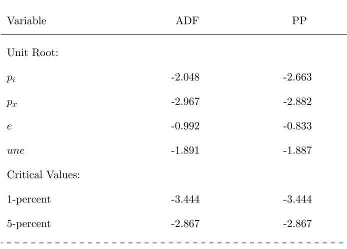
Having identified the series to be used in the empirical analysis, it is useful to examine some of
their basic statistical properties. Specifically, we test each series for the null of a unit root by
using augmented Dickey–Fuller (ADF) and Phillips–Perron (PP) tests (Dickey and Fuller, 1979;
Phillips and Perron, 1988). In implementing the ADF test, we account for the potential effects of
heteroskedasticity by using the modified test statistic suggested by Demetrescu (2010). As well,
we choose lag lengths for the autoregressive parameters in the ADF test by using the lag–length
selection procedures outlined by Ng and Perron (1995); for the PP test we choose a lag length based
on the rule int(4(T /100)0.25, which is six in the present case. The results are reported in upper
panel of Table 1.
As recorded in the Table, the tests provide evidence of nonstationarity for each variable
consid-ered.7 In terms of the conceptual framework outlined in the previous section, the implication is that
equation (7) should now be viewed as a cointegrating regression, and thereby reflects the long–run
relationship the two price variables and the exchange rate variable. Following Balke and Fomby
(1997), we estimate the (unrestricted) version of (7) and test the resulting residual series for the
presence of a unit root. The results in this instance are reported in the lower panel of Table 1.
Regardless of which test is employed (i.e., ADF or PP), it is clear that we reject the unit root
hypothesis and conclude that the prices and the exchange rate are cointegrated. This information
will be fundamental in specifying and estimating the subsequent nonlinear model used to estimate
ERPT effects, to which we now turn.
4 Modeling Framework
4.1 Multivariate Smooth Transition Models
To explore the the exchange rate pass–through effects for Canadian and U.S. prices, we
fol-low prior literature in specifying a (nonlinear) vector error correction model (VECM) (see, e.g.,
Al-Abri and Goodwin, 2009). Specifically, the basic building block of our empirical analysis is a
7
VECM model of the general form:
∆yt=δ+
p−1
∑
i=1 Ψ
ΨΨi∆yt−i+αεˆt−1+υt, (9)
where yt = (pit, pxt, et)′; ˆεt−1 is the lagged residual from the cointegrating regression described
in the previous section, that is, the (lagged) departure from long–run equilibrium; δ and α are
conformable parameter vectors, whereαcontains the so called speed–of–adjustment parameters or
error correction coefficients; ΨΨΨi are conformable parameter matrices; and υt is a vector of mean
zero, random, additive errors.
If nonlinear ERPT effects are not considered, then the system in (9) can be estimated and
im-pulse response functions generated in order to determine the degree or pass–through. Alternatively,
if nonlinearities of the sort described in previous sections are considered, then it is necessary to
modify (9). In the spirit of the regime switching framework in (8), we could re–specify the VECM
as:
∆yt =
[
δ1+ p−1
∑
i=1 Ψ
ΨΨi1∆yt−i+α1εˆt−1
]
(1−G(st,θ))
+
[
δ2+ p−1
∑
i=1 Ψ
ΨΨi2∆yt−i+α2εˆt−1
]
G(st,θ) +υt, (10)
where ∆ is a difference operator such that ∆xt=xt−x‘t−1. In (10) the functionG(.), the so called
transition function, now plays the role of the Heaviside indicator function defined previously andθis
now a vector of parameters that identifies the transition function. Importantly, similar to the
Heav-iside indicator function, the functionG(.) is bounded between zero and one. A primary difference,
however, is thatG(.) can also assume intermediate values on the unit interval, that is, regime change
can be potentially gradual or smooth. For this reason the model in (10) is referred to as a smooth
transition VECM, or STVECM, and was introduced originally by Rothman, van Dijk and Franses
(2001). Furthermore, the STVECM is a straightforward extension of the univariate smooth
tran-sition autoregressive (STAR) models introduced originally by Ter¨asvirta (1994). The model is, of
course, nonlinear in parameters given thatγ andcmust also be estimated, and therefore nonlinear
To implement the STVECM it is necessary to specify a form for the transition function, G(.).
In the present case if, for example, it is hypothesized that ERPT varies with the magnitude of the
departure from long–run equilibrium, then it would be feasible to specify the transition function
as:
G(st;γ, c) = 1−exp
(
−γ(st−c)2
/
ˆ
σst2), (11)
that is, the exponential distribution, whereθ = (γ, c),γ being the speed–of–adjustment parameter
and c being the centrality parameter; and ˆσst is the sample standard deviation of the transition
variable, st. In (11) as the transition variable, st, approaches c the function G(.) approaches zero
while, conversely, when st deviates far fromc the functionG(.) approaches unity. The speed with
which the transition from one extreme to the other occurs is dictated by the magnitude of the
parameter, γ. In this manner the exponential function is capable of approximating something
akin to a three–regime threshold model of the sort employed by Al-Abri and Goodwin (2009) and
Larue, Gervais and Rancourt (2010), albeit in a potentially smooth way. To abbreviate, we refer to
a regression equation with an exponential transition function as an exponential smooth transition
regression equation, or ESTR.
Alternatively, the logistic function, specified as:
G(st;γ, c) = [1 + exp (−γ(st−c)/ˆσ)]−1, (12)
is an another widely used specification for the transition function, G(.), in the STVECM (see, e.g.,
Rothman, van Dijk and Franses, 2001). In (12) as st increases above the centrality parameter c,
the functionG(.) will approach unity. Alternatively, forstbelowcthe logistic function approaches
zero. Again, the speed with which this transition occurs is determined by the relative magnitude of
the parameterγ. By incorporating (12) into (10), it follows that the resulting STVECM can display
asymmetric behavior depending on the value of the transition variable,st. For example, one option,
and one largely unexplored in the ERPT literature, is to setst equal to some observed measure of
real economic activity such as the unemployment rate in an attempt to mimic the business cycle.
Here we refer to a regression equation that uses a logistic transition function as a logistic smooth
As specified in (10), it follows that each equation in the STVECM will share the same (identical)
transition function. This is the approach most commonly applied in the literature; see, for example,
Anderson and Vahid (1998), Rothman, van Dijk and Franses (2001) and Camacho (2004). From
an empirical perspective such a specification may be overly restrictive. In other words, it is entirely
possible thatpit will respond tostwith a different speed than willpxt. Of course it is even possible
that the various equations in the system will have completely different transition functions, that
is, some mix of logistic and exponential functions. In this spirit it is a straightforward matter to
generalize (10) as follows:
∆yt = (III−ΓΓΓt)
[
δ1+ p−1
∑
i=1
ΨΨΨi1∆yt−i+α1εˆt−1
]
+ ΓΓΓt
[
δ2+ p−1
∑
i=1
ΨΨΨi2∆yt−i+α2εˆt−1
]
+υt, (13)
whereIII is a 3×3 identity matrix and diag (ΓΓΓt) = (G1(s1t), G2(s2t), G3(s3t)), with off diagonal terms
equalling zero. In this manner the STVECM in (10) may be generalized to allow for different
transi-tion functransi-tions (and transitransi-tion variables) for each equatransi-tion in the system. He, Ter¨asvirta and Gonz´alez
(2008) considered a similar specification for a vector–autoregressive model, although they limited
their analysis to the case where st simply equals the time index, t.
To our knowledge the STVECM framework has not been used to model regime dependent
exchange rate pass–through effects. This is surprising given that the STVECM clearly nests many
of the more common specifications used to examine nonlinear responses in the empirical literature
on exchange rate pass–through.
4.2 A Testing Strategy: Single Equations
As is evident from both (10) and (13), the nonlinear features of the provisional STVECM model
will depend on the selection of the transition function(s) as well as the transition variable(s). In
practice there are typically a large number of options available during the model building phase.
It is therefore desirable to have a testing strategy that reduces the number of nonlinear models
that must ultimately be estimated and compared. To date there has been relatively little research
equation models (Ter¨asvirta, 1994; Lundbergh, Terasvirta and van Dijk, 2003).
To gain insight into the testing problem, consider for the moment the case where (10) is reduced
to a univariate smooth transition error correction model, that is, whereyt= ˜yt is a scalar. In this
case we can re–write (10) as:
∆˜yt=ϕ′1x˜t(1−G(st;θ)) +ϕ′2x˜tG(st;θ) +υt, (14)
wherex˜t=(1,∆y′t−1, . . . ,∆yt′−p+1,εˆt−1)′, a (3×p+1) vector, and whereϕ1andϕ2are conformable
parameter vectors. As well, assume that G(.) is given by either (11) or (12). The problem, of
course, is there are two ways to reduce (14) to a linear error correction model. On the one hand if
ϕ1 =ϕ2, then the model becomes linear in parameters. Even so, it is not appropriate to simply
test H0 :ϕ1 =ϕ2 given that in this case theγ andcparameters embedded inG(.) are unidentified.
Likewise, a standard test of H0 :γ = 0 is not appropriate given that in this case ϕ1 and ϕ2 are
unidentified. The result in either case is the classical “Davies problem” outlined in a pair of papers
by Davies (1977; 1987). The upshot is that tests of either null hypothesis will be associated with
non–standard asymptotic distributions.
While various testing procedures have been proposed, a computationally convenient approach
has been proposed by Luukkonen, Saikkonen and Ter¨asvirta (1988). Specifically, these authors
advocate replacing the transition function G(.) with a suitable Taylor series approximation, where
the approximation is evaluated atγ = 0. If, for example, a third–order approximation is used, then
a linear approximation to (14) is:
∆˜yt=ψ′1x˜t+ψ2′x˜tst+ψ3′x˜ts2t +ψ4′x˜ts3t +ξt. (15)
A test of linearity may now be conducted by simply testing H′0 :ψ2 =ψ3 =ψ4 =0 in (15). Note
that while in general ξt contains both εt and approximation error, under the null hypothesis of
linearity there is no approximation error. In this case εt = ξt, and standard Lagrange Multipler
(LM) tests such including the F–test may be applied. That is, if RSS1 denotes the error sum of
unrestricted model, then:
FLM =
(RSS1−RSS2)/q
RSS2/(n−k)
approx
∼ F(q, T −p−1), (16)
whereq = 3(p+ 1) are the number of restrictions implied by the null hypothesis H′0 and and kare
the number of free parameters estimated in the unrestricted version of (15).
While the foregoing outlines a reasonable testing strategy for detecting nonlinearity, several
issues remain. For example, it does not directly determine which transition function, that is, the
exponential or the logistic, is most appropriate for a given application. Moreover, the nonlinearity
test assumes that the transition variable, st, is known. While in some instances theory might
dictate a likely candidate for transition variable, in many instances this choice, too, must be part
of the overall testing framework. Regarding the first issue, Ter¨asvirta and Anderson (1992) and
Ter¨asvirta (1994) describes a testing sequence that can be employed to identify the transition
function. Specifically, assuming the linear model is rejected, the following conditional tests may be
performed:
H04: ψψψ4 = 000, (17)
H03: ψψψ3 = 000|ψψψ4= 000, (18)
H02: ψψψ2 = 000|ψψψ3=ψψψ4= 000, (19)
where again it is appropriate to use suitable F–versions of the tests implied by (17)–(19). The
logic of the above testing sequence is that an exponential function is likely best approximated
by a quadratic in st. Therefore, if (18) is rejected while (17) and (19) are not, the exponential
function in (11) may be used. Alternatively, if (17) or (19) are rejected while (18) is not, than
the logistic function in (12) may be tried.8 Finally, there are few restrictions on candidates for
the transition variable, st. Again, Ter¨asvirta (1994) suggests trying a slate of candidates and
using the one associated with the strongest rejection of the linearity hypothesis, H′0. Finally,
once a candidate transition variable and transition function have been identified, provisional
es-8
timates of the smooth transition model in (14) can be obtained by employing nonlinear least
squares (van Dijk, Ter¨asvirta and Franses, 2002). Furthermore, the diagnostic tests described by
Eitrheim and Ter¨asvirta (1996) can be employed to examine model adequacy.
4.3 A Testing Strategy: Multivariate Systems
As noted previously, there is a paucity of studies that have explored nonlinearity testing in a
mul-tivariate setting, especially when a system such as (13) is examined with equation–specific transition
functions. Even so, Rothman, van Dijk and Franses (2001), Camacho (2004), and P´eguin-Feissolle, Strikholm and T
(2008) are notable exceptions, with each of these studies advancing a framework for testing
non-linearities in a multi–equation model. In principle doing so is straightforward: the multivariate
counterpart to (15) may be specified as:
∆yyyt=̥̥̥1XXXt+̥̥̥2XXXtsss1t+̥̥̥3XXXtsss2t+̥̥̥4XXXtsss3t+ξξξt, ξξξt∼N(000,ΣΣΣ), (20)
where in this caseXtis a 3×(p+ 1) matrix defined asXXXt=ιιιxxx˜˜˜′t, and whereιιιis a (3×1) unit vector.
As well,sssit =
(
si
1t, si2t, si3t
)′
,i= 1,2,3,̥̥̥i,i= 1, . . . ,4, are conformable parameter matrices, and
where ΣΣΣ is a symmetric, positive–definite error covariance matrix. The system nonlinearity test
then involves a test of the hypothesis H′′0 :̥̥̥2 =̥̥̥3=̥̥̥4 = 0, which will involveq= 3 [3×(p+ 1)]
linear restrictions on the parameters of (20).
Following Bewley (1986), anF–version of the LM test of H′′0 in the multi–equation system is:
FLM S =
T q
(
m−tr(ΩΩΩˆ1ΩΩΩˆ
−1 0
))approx
∼ F(q, T), (21)
where ΩΩΩ0 =TΣΣΣˆ0 with ˆΣΣΣˆˆ0 being the estimated residual covariance matrix for the model under the
null, ΩΩΩ1 = TΣΣΣˆˆˆ1 similarly defined for the model under the alternative, and m is the number of
equations in the system (herem= 3). While a value forFLM S that exceeds the critical value from
the F(q, T) distribution is a clear indication of nonlinearity in the system, it says nothing about
which equation(s) are appropriately nonlinear, nor does it suggest which transition function or set
of transition variables are most applicable.
While as such a richer, more detailed sequence of tests could be developed, the fact is the number
of combinations of candidate transition variables and transition functions involved could quickly
become overwhelming. We therefore propose a simple yet practical strategy for identifying the
appropriate form of the STVECM in (13). Specifically, we propose using the single–equation
testing framework outlined in the previous section for specifying the structure of each equation in
the system. Furthermore, once a set of candidate transition variables has been identified, the test
in (21) may be employed to evaluate system–wide nonlinearity.
5 Empirical Results
5.1 Nonlinearity Testing Results
The testing and estimation methods described above are used to examine nonlinearity in exchange
rate pass–through for U.S. and Canadian OSB prices. The approach first necessitates estimating
a best–fitting linear error correction model for each equation. The explanatory variables used are
lags of (first differences) of representative (logarithmic) OSB import and export prices and the first
difference of the log of the U.S. dollar–Canadian dollar exchange rate. A systems version of Akaike’s
information criterion (AIC) is used to determine appropriate lag lengths.9 The AIC indicated that
up to four lags of the ∆yt vector are needed in each equation. Even so, two additional lags were
called for to render the residuals of the foreign exchange equation white noise. Additional testing
confirmed that exchange rates respond only to their own lags, and are therefore exogenous to OSB
prices. As well, preliminary tests suggested that lagged changes in exchange rates are insignificant
in the OSB price equations.10
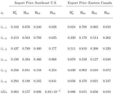
The results of nonlinearity tests applied to the U.S. and Canadian OSB price equations are
reported in Table 2. Candidates for the transition variables include up to six lags of the lagged
residual from the estimated cointegrating equation (i.e., ˆεt−j, j= 1, . . . ,6) and a 52–week moving
9
Specifically, we use AIC =ln(det( ˆΣ))+ 2N/T, whereN denotes the number of estimated parameters in the model.
10
average of the unemployment rate, that is,
g
unet =
1 52
52
∑
i=1
unet−i. (22)
The fifty–two week average smooths out short–term and seasonal fluctuations in the weekly
un-employment rate, and therefore should over time send a reasonable signal of general economic
conditions. The test results show that for both equations, linearity is most convincingly rejected
for the unegt variable. Moreover, the results of applying the testing sequence in (17)–(19) suggest
that the transition function is likely a logistic as specified in (12). The implication, then, is that
ERPT into OSB prices is likely asymmetric, and moreover that this asymmetry occurs in
conjunc-tion with a general indicator of the business cycle. This preliminary result is, moreover, consistent
with recent work by Chew, Ouliaris and Tan (2011).
At this stage several additional issues must be considered. First is the question of what transition
variable is most likely associated with nonlinearity in the exchange rate equation, which contains an
intercept and six lags of the log difference of exchange rates. To this end, the nonlinearity tests were
repeated for the exchange rate equation; the results are reported in the left–hand panel of Table
3. Of the transition variables considered, results in Table 3 indicate the presence of substantial
nonlinearities in the exchange rate equation, with st = ∆et−1 being associated with the strongest
rejection of linearity. And for this variable the testing sequence suggests that an LSTR might be
the most appropriate specification, although the rejection of H03 is also quite strong, indicating
that an ESTR specification could also be acceptable.
The preliminary evidence reported above suggests that a 52–week moving average of
unemploy-ment is a reasonable transition variable in both OSB price equations. Therefore, it may be desirable
to incorporate a fourth equation into the system to explain weekly unemployment rates. Moreover,
prior work–see, for example, van Dijk, Ter¨asvirta and Franses (2002) and Deschamps (2008)–has
found substantial evidence in favor of LSTR models for monthly U.S. unemployment rates. Even
so, to our knowledge prior studies have not focused on modeling unemployment rates (based on
unemployment claims) on a weekly basis. The base linear model used here is of the form:
∆eyt=λ0+ 3
∑
i=1
(ηisin (2πt/fi) +κicos (2πt/fi)) + p−1
∑
i=1
where yet = unet and f1 = 13, f2 = 26, and f3 = 52. The sine–cosine terms are incorporated to
account for the seasonal nature of unemployment claims. As well, we follow Skalin and Ter¨asvirta
(2002) by including a lagged level term for the unemployment variable, which in turn implies
that unemployment follows a “natural rate” (i.e., is mean reverting) as opposed to a “hysteresis”
hypothesis.11 Of course once nonlinearities are considered, it is possible that unemployment rates
could even display locally explosive behavior.
The linear model in (23) was fitted to the data. The (univariate) AIC indicated that up to eleven
lags of ∆unetare needed to eliminate residual serial correlation. Results of applying linearity tests
for the unemployment rate equation are recorded in the right–hand panel of Table 3. Consistent
with prior studies, as well as with the asymmetries that may be detected by simply the data plot
in Figure 3, there is overwhelming evidence of nonlinearity in the unemployment data. Results
in Table 3 suggest that linearity is rejected most convincingly for(unet−1−unet−4). Of interest
is that the seasonal difference (unet−1 −unet−53) and the 52–week moving average unegt, while
indicating the presence of nonlinearities, are not the strongest candidates for a transition variable
in the unemployment equation.12 In all instances the testing sequence overwhelmingly indicates
that an LSTR model is called for, a result that is, moreover, also consistent with prior research
(van Dijk, Ter¨asvirta and Franses, 2002).
5.2 Smooth Transition Model Results
The foregoing suggests there is evidence of nonlinearity in each equation in the system, which
among other things suggests that ERPT into OSB prices may have a regime–dependent effect. As
discussed in Section 4, as part of the STVECM model building process we first estimate suitable
univariate smooth transition models for each equation.
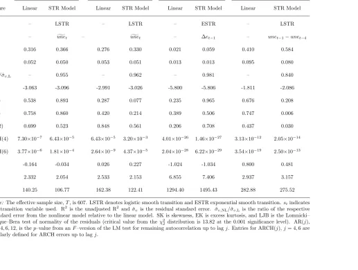
The results of the univariate analysis are summarized in Table 4–there we report model fit
diagnostic measures for each of the estimated linear and nonlinear models for each variable in the
system. To begin, preliminary estimations revealed that an LSTR specification for the exchange
11
Of course the results reported in Table 1 suggest thatunet behaves in a manner consistent with a unit root process (i.e., hysteresis). Even so, Skalin and Ter¨asvirta (2002) report that it is often difficult reject the null of a unit root even when the underlying data were generated in a manner consistent with mean–reverting behavior and strong asymmetries.
12
rate equation (that uses st= ∆yt−1 as a transition variable) ended up fitting only a small handful
of outliers. Given the results in Table 3, we also fitted an ESTR to the exchange rate series, which
yielded more satisfactory results. Turning to an assessment of the univariate models, results in
Table 4 show that in every case the nonlinear model represents an improvement in fit relative to its
linear counterpart, with the nonlinear unemployment equation yielding the biggest increase in fit
relative to its linear counterpart and the exchange rate equation the smallest. In addition, there is
little evidence of remaining autocorrelation in each model’s residuals up to a twelve–week lag (the
smooth transition model for unemployment at lags six and twelve being an exception). Results in
Table 4 also indicate that the residuals for each estimated model are highly leptokurtic (i.e., they
are associated with “fat tails”), which is not surprising given the relatively high frequency of the
data (weekly). There is also evidence of ARCH errors in each case, a result that, moreover, might
be anticipated given the weekly frequency of the data.
As a final check of the nonlinear specifications, the system nonlinearity test, as outlined in (21),
was applied to the four–equation system. In conducting the test the system in (20) was estimated
where the transition variables identified for the univariate models in Table 4 are used. The resulting
test statistic, 2.690, is extreme in the corresponding F(132,607) distribution. Taken together, this
result and those recorded in Table 4 suggest that nonlinearity is an important feature of these data.
The final step in constructing a model for assessing regime–dependent ERPT into North
Amer-ican OSB prices is to estimate the STVECM. The transition functions and transition variables
used in specifying the univariate models are maintained; the parameter estimates obtained for the
univariate models are used as starting values. The system estimation results, along with several
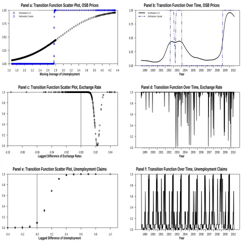
summary measures of model fit, are reported in Table 5. Plots of the corresponding estimated
transition functions for each equation, both over time and with respect to each implied transition
variable, are reported in Figure 4. Additional tests revealed that covariance terms amongst the
price variables and exchange rates and unemployment were not significantly different from zero,
as is the covariance term between the exchange rate and unemployment. These restrictions are
incorporated in the estimates recorded for the STVECM reported here.
As indicated in Table 5, the STVECM provides a substantial improvement in fit relative to
the linear VECM; for example, the ratio of the determinant for the STVECM’s covariance matrix
in fit for the STVECM relative to the linear VECM. Regarding the implied nonlinearities, the plots
in Figure 4 show that, with the exception of the transition function for the OSB price in Eastern
Canada, the estimated transition functions imply a smooth response to changes in the respective
transition variables. The plots in Figure 4 also suggest that the transition functions for the OSB
price equations, when plotted over time, do a reasonable job of tracking recent business cycle
behavior. Finally, the parameter estimates reported in Table 5 suggest that, for each estimated
equation, the estimated parameters change substantially with respect to the implied transition
functions, including the speed–of–adjustment parameters associated with the lagged error correction
terms in the OSB price equations. Furthermore, the STVECM apparently does a reasonable job
of generating results for prices, the exchange rate, and the unemployment rate that are consistent
with observed behavior. Along with the observed data, Figures 2 and 3 show the realizations of
a single Monte Carlo simulation of the model from the end of the sample period (August, 2010)
through the middle of 2014. In each case the simulated data seemingly depicts various features of
the observed data, including asymmetries. Taken together, the results for the estimated STVECM
suggest there is scope for ERPT into OSB prices to vary with the weekly U.S. unemployment rate
and that, moreover, unemployment itself is also a highly nonlinear process.
5.3 Generalized Impulse Response Functions
To assess the effects of ERPT into OSB prices, it is useful to generate generalized impulse response
functions (GIRFs). Specifically, Koop, Pesaran and Potter (1996) define a set of procedures that
may be applied to compute GIRFs for multivariate nonlinear models. A (multivariate) GIRF is
defined by:
G∆y(n,δ,ωt−1) =E(∆yt+n|υt=δ,Ωt−1 =ωt−1)−E(∆yt+n|υt=0,Ωt−1 =ωt−1), (24)
where n denotes the forecast horizon, δ is a vector of shocks, Ωt−1 = ωt−1 denotes information
available through period t−1 (i.e., the history), and E is an expectation operator. To
deter-mine the initial conditions, we randomly draw (with replacement) 50 histories (i.e., ωt−1’s) from
the set of 607 available histories. As is common in the ERPT literature, we then consider unit
unemployment rate. To evaluate the expectations in (24), we use 600 Monte Carlo draws from a
multivariate random normal distribution with a variance–covariance matrix equal to that of the
estimated STVECM. Impulse responses for the levels of the variables in the system are computed
by summing those obtained for the first differences, that is, by constructing:
Gy(n,δ,ωt−1) = n
∑
i=1
G∆y(n,δ,ωt−1). (25)
Finally, it is also possible to construct regime–dependent GIRFs where, for example, shocks can be
initiated only when G1(s1t) ≥0.5 or G1(s1t)<0.5.13 In this manner it is possible to examine the
extent to which ERPT into OSB prices varies with the unemployment rate.
Unconditional GIRFs for a one–time unit shock (both positive and negative) to the U.S. dollar–
Canadian dollar exchange rate, taken over a 156–week horizon, are reported in Figure 5. As
illustrated there, pass–through of such a shock into the U.S. OSB price is never complete, reaching
at most 75–percent. Moreover, the effects are initially quite small–they do not reach even 50–
percent during the first year following the shock. As well, the GIRFs appear to be symmetric with
respect to positive versus negative exchange rate shocks. This result is reasonable given that: (1)
unemployment is not impacted by nominal exchange rate movements (and therefore there is no
systematic “regime change” for the OSB price equations); and (2) that nonlinearity in the exchange
rate equation is associated with an ESTR, which is (nearly) symmetric around zero.
A different picture emerges, however, when conditional GIRFs are computed for an exchange
rate shock; see Figure 6. As the figure shows, when the 52–week moving average of unemployment
(i.e.,s1t) is greater than 2.91–percent, that is, whenG1(s1t)≥0.5, ERPT associated with a positive
one–unit shock reaches unity (i.e., is complete) after only twelve weeks. Indeed, as depicted in Figure
6, this stabilizes at a value far in excess of unity–near three, in fact–after approximately two years
have elapsed. Conversely, the GIRFs conditional on the moving average of unemployment being
less than 2.91–percent (i.e., G1(s1t) <0.5) illustrate that pass–through is, again, slow to respond
and, moreover, relatively incomplete, even after three years have elapsed; the long–run response to
a positive unit shock in this case is about 0.44–percent. These results firmly establish that ERPT
into prices for a primary home construction material, that is, oriented strand board, is highly regime
13
Given the estimate for the centrality parameter,c1, reported in Table 5, the conditional GIRFs in this case are
dependent and that, moreover, the regimes themselves are a function of the overall performance of
the general economy.
Because of the nature of the model it is also possible to obtain GIRFs associated with an
unem-ployment shock, in this case with respect to a one standard deviation shock to the unemunem-ployment
rate. The resulting unconditional GIRFs are reported in Figure 7. They show, for example, that a
positive shock to unemployment apparently causes unemployment rates themselves to continue to
rise throughout the three–year horizon. As well, the impact on OSB prices is initially positive but
after approximately 100 weeks the effects become negative. Furthermore, the GIRFs in Figure 7
that the estimated STVECM is apparently not dynamically stable with respect to unemployment
shocks, as the GIRFs for prices and unemployment do not stabilize at a new level. This is not
the case, however, as revealed in Figure 8. There we see the GIRF for unemployment (in response
to an unemployment rate shock) extended over a six–year horizon. What is revealed there is that
after approximately six years have elapsed that the GIRFs for unemployment effectively return to
zero. In short, the model depicts something akin to a six–year peak–to–peak business cycle (based
on unemployment), a result that is, moreover, in keeping with the general conclusion that post–war
business cycles in the United States have lasted, on average, for approximately five–six years (see,
.e.g., Watson, 1994).
As before, it is possible to obtain conditional GIRFs for unemployment shocks, in this case
when G4(s4t) ≥ (respectively <) 0.5. The results for these conditional GIRFs are reported in
Figure 9. Among other things the plots in Figure 9 bring into focus the asymmetries associated
with unemployment. To begin, the effects on the U.S. price for OSB associated with a positive
shock are, as before, initially positive, although the peak occurs much more quickly when st4 =
unet−1−unet−4≥0.149, that is, when unemployment rates are trending higher (25 weeks versus
approximately 45 weeks). Even so, the effects resulting from a positive shock apparently converge
after approximately 100 weeks. More interesting, however, is that negative shocks yield GIRFs
that are always larger in absolute terms when G4s4t ≥ 0.5 as opposed to when G4s4t ≥ 0.5.
Apparently a decrease in unemployment has a larger effect on OSB prices when unemployment
rates are, relatively speaking, already high than when the converse is true. Similar results occur for
the conditional GIRFs associated with the Canadian OSB price associated with an unemployment
6 Summary and Conclusions
In this study we have examined exchange rate pass–through into oriented strand board, an
im-portant construction material produced and traded throughout much of North America. Indeed,
Canada and the United States are leading producers of OSB, but historically Canada has exported
more than 75–percent of its total OSB production to the United States. In the U.S. OSB is
pro-duced primarily in the Southeastern region of the country, although in recent decades this region
has also experienced the most rapid growth (and, since 2007, the most rapid declines) in new home
construction. To investigate ERPT into OSB prices, we obtained weekly mill–gate prices from
Ran-dom Lengths for the 1998–2010 period. Specifically, the prices correspond to mill prices for OSB in
Eastern Canada (prices for mills in Ontario and Quebec) and the Southeast U.S. (prices for mills in
Georgia, Alabama, Mississippi, South Carolina, and Tennessee). Furthermore, the Canadian prices
are recorded in U.S. dollars, that is, local currency pricing is employed.
Recent work by Goodwin, Holt and Prestemon (2011) found evidence of nonlinearity in the
LOP relationship between these prices, but they did not consider ERPT effects. Moreover, recent
research has examined nonlinear and asymmetric ERPT into import prices by assuming that
de-viations from the underlying long–run equilibrium relationship will have a differential impact on
estimated pass–through responses depending on the overall dagnitude of the deviations (see, e.g.,
Al-Abri and Goodwin, 2009; Larue, Gervais and Rancourt, 2010). More recently, several authors
have investigated asymmetric effects of ERPT into prices as a function of overall macroeconomic
ac-tivity (Nogueira, Jr. and Le´on-Ledesma, 2011; Chew, Ouliaris and Tan, 2011), albeit for aggregate
price indices and not for specific industries or commodity prices.
Building on prior work in this general area, we examine the asymmetric effects of long–term
swings in weekly unemployment claims on ERPT into prices for OSB. We do so by proposing
a feasible strategy for building and estimating a smooth transition vector error correction model
wherein each equation is allowed to have its own built–in asymmetries (i.e., transition function and
transition variables). Specifically, we estimate a four–equation STVECM where asymmetries in
the the OSB price equations are modeled by using logistic transition functions where, moreover,
the transition variables are in both cases a 52–week moving average of the unemployment rate.
exponential transition function. And finally, in a manner consistent with prior work on modeling
asymmetries in unemployment rates (see, e.g., Skalin and Ter¨asvirta, 2002), we model asymmetries
in weekly unemployment rates by using a logistic smooth transition model.
An immediate implication of the estimated STVECM is as follows: not only is there the potential
for direct asymmetric (nonlinear) ERPT into OSB prices, but also the potential for indirect effects
due to the regime–dependent behavior identified separately for the exchange rate and unemployment
equations. To our knowledge no prior study has allowed for such a rich specification of nonlinearities
when examining ERPT. To assess the nature of nonlinearities in ERPT, we employ the generalized
impulse response function framework of Koop, Pesaran and Potter (1996). Similar to prior work on
this general topic, we find incomplete pass–through into OSB prices in both the U.S. and Canada.
Moreover, for OSB prices in the Southeast U.S., pass–through effects are very small in the short
run and only reach a long–run steady state of approximately 0.75 (for a positive shock) after more
than two years have elapsed. As well, these estimated effects depend in a striking way on overall
macroeconomic conditions. Specifically, conditional GIRFs, that is, GIRFs obtained for when
unemployment rates are high versus low, indicate that ERPT effects during the recent economic
downturn were far greater than unity. These results are, moreover, in keeping with prior work
by Nogueira, Jr. and Le´on-Ledesma (2011) and Chew, Ouliaris and Tan (2011), who also find that
pass–through effects increase substantially during economic downturns. Finally, because of the
way the STVECM is specified, we can also examine GIRFs associated with unemployment shocks,
that is, unemployment pass–through effects. We find these effects are generally smaller than for
exchange rate shocks, although they vary considerably over a six–seven year period, which in turn
is roughly consistent with the observed span for post–war business cycle activity.
While this paper represents an important contribution to the ERPT literature, and especially
so for timber products, more work remains. Specifically, it would be useful to examine the potential
asymmetric responses to other measures of macroeconomic activity. As well, it would be desirable
to repeat the analysis for price relationships involving other products and trade to–from other
countries and regions. Even so, we believe the work reported here provides a good starting point
References
Al-Abri, Almukhtar S. and Barry K. Goodwin, “Re–examining the Exchange Rate Pass– through into Import Prices using Non–linear Estimation Techniques: Threshold Cointegration,”
International Review of Economics & Finance, January 2009, 18(1), 142–161.
Anderson, Heather M. and Farshid Vahid, “Testing Multiple Equation Systems for Common
Nonlinear Components,”Journal of Econometrics, May 1998, 84(1), 1–36.
Bailliu, Jeannine and Eiji Fujii, “Exchange Rate Pass–Through and the Inflation Environment in Industrialized Countries: An Empirical Investigation,” Working Papers 04-21, Bank of Canada 2004.
Balke, Nathan S. and Thomas B. Fomby, “Threshold Cointegration,”International Economic Review, August 1997,38 (3), 627–645.
Bewley, Ron,Allocation Models, Cambridge, Massachusetts: Ballinger Publishing Company, 1986.
Bolkesjø, Torjus F. and Joseph Buongiorno, “Short- and Long-Run Exchange Rate Effects
on Forest Product Trade: Evidence from Panel Data,”Journal of Forest Economics, 2006, 11
(4), 205–221.
Bussiere, Matthieu, “Exchange Rate Pass–Through to Trade Prices – The Role of Non– Linearities and Asymmetries,” Working Paper Series 822, European Central Bank October 2007.
Camacho, Maximo, “Vector Smooth Transition Regression Models for US GDP and the
Com-posite Index of Leading Indicators,”Journal of Forecasting, 2004, 23(3), 173–196.
Campa, Jos´e Manuel and Linda S. Goldberg, “Exchange Rate Pass–Through into Import
Prices,”The Review of Economics and Statistics, December 2005, 87(4), 679–690.
Campa, Jos´e Manuel, Linda S. Goldberg, and Jose M. Gonzalez-Minguez, “Exchange Rate Pass–Through to Import Prices in the Euro Area,” Staff Reports 219, Federal Reserve Bank of New York 2005.
Cashin, Paul, Hong Liang, and C. John McDermott, “How Persistent Are Shocks to World
Commodity Prices?,”IMF Staff Papers, 2000, 47(2), 177–217.
Chew, Joey, Ouliaris, and Siang Meng Tan, “Exchange Rate Pass–Through over the Business Cycle in Singapore,” IMF Working Papers 11/141, International Monetary Fund June 2011. http://ideas.repec.org/p/imf/imfwpa/11-141.html.
Davies, R. B., “Hypothesis Testing When a Nuisance Parameter is Present Only Under the
Alternative,”Biometrika, 1977, 64(2), pp. 247–254.
Davies, Robert B., “Hypothesis Testing when a Nuisance Parameter is Present Only Under the
Alternatives,”Biometrika, 1987, 74(1), pp. 33–43.
Demetrescu, Matei, “On the Dickey–Fuller Test with White Standard Errors,”Statistical Papers,
January 2010, 51(1), 11–25.
Deschamps, Philippe J., “Comparing Smooth Transition and Markov Switching Autoregressive
Dickey, David A. and Wayne A. Fuller, “Distribution of the Estimators for Autoregressive
Time Series With a Unit Root,”Journal of the American Statistical Association, 1979,74(366),
pp. 427–431.
Eitrheim, Øyvind and Timo Ter¨asvirta, “Testing the Adequacy of Smooth Transition
Autore-gressive Models,”Journal of Econometrics, September 1996, 74(1), 59–75.
Gagnon, Joseph E. and Jane Ihrig, “Monetary Policy and Exchange Rate Pass–Through,”
International Journal of Finance & Economics, 2004, 9 (4), 315–338.
Goldberg, Pinelopi Koujianou and Michael M. Knetter, “Goods Prices and Exchange Rates:
What Have We Learned?,”Journal of Economic Literature, September 1997, 35(3), 1243–1272.
Goodwin, Barry K., Matthew T. Holt, and Jeffrey P. Prestemon, “North American Oriented Strand Board Markets, Arbitrage Activity, and Market Price Dynamics: A Smooth
Transition Approach,”American Journal of Agricultural Economics, 2011, 93(4), 993–1014.
He, Changli, Timo Ter¨asvirta, and Andreas Gonz´alez, “Testing Parameter Constancy in
Stationary Vector Autoregressive Models Against Continuous Change,” Econometric Reviews,
2008, 28(1–3), 225–245.
Jabara, Cathy L. and Nancy E. Schwartz, “Flexible Exchange Rates and Commodity Price
Changes: The Case of Japan,”American Journal of Agricultural Economics, 1987,69 (3), 580–
590.
Karoro, Tapiwa D., Meshach J. Aziakpono, and Nicolette Cattaneo, “Exchange Rate
Pass–Through to Import Prices in South Africa: Is there Asymmetry?,”South African Journal
of Economics, 2009, 77(3), 380–398.
Knetter, Michael M., “Price Discrimination by U.S. and German Exporters,”The American Economic Review, 1989, 79(1), 198–210.
Koop, Gary, M. Hashem Pesaran, and Simon M. Potter, “Impulse Response Analysis in
Nonlinear Multivariate Models,”Journal of Econometrics, September 1996, 74(1), 119–147.
Larue, Bruno, Jean-Philippe Gervais, and Yannick Rancourt, “Exchange Rate Pass–
Through, Menu Costs and Threshold Cointegration,”Empirical Economics, 2010, 38, 171–192.
10.1007/s00181-009-0261-2.
Leamer, Edward E., “Housing IS the Business Cycle,” NBER Working
Pa-pers 13428, National Bureau of Economic Research, Inc September 2007.
http://ideas.repec.org/p/nbr/nberwo/13428.html.
Lundbergh, Stefan, Timo Terasvirta, and Dick van Dijk, “Time–Varying Smooth Transition
Autoregressive Models,”Journal of Business & Economic Statistics, January 2003, 21(1), 104–
21.
Luukkonen, Ritva, Pentti Saikkonen, and Timo Ter¨asvirta, “Testing Linearity Against
Smooth Transition Autoregressive Models,”Biometrika, 1988, 75(3), 491–499.
Magee, Lonnie, “R2 Measures Based on Wald and Likelihood Ratio Joint Significance Tests,”The American Statistician, 1990,44(3), 250–253.
Mann, Catherine L., “Prices, Profit Margins, and Exchange Rates,” Federal Reserve Bulletin, 1986, (Jun), 366–379.
Marazzi, Mario and Nathan Sheets, “Declining Exchange Rate Pass–through to U.S. Import
Prices: The Potential Role of Global Factors,” Journal of International Money and Finance,
2007, 26(6), 924–947.
Ng, Serena and Pierre Perron, “Unit Root Tests in ARMA Models with Data-Dependent
Methods for the Selection of the Truncation Lag,”Journal of the American Statistical Association,
1995, 90(429), 268–281.
Nogueira, Jr., Reginaldo P. and Miguel A. Le´on-Ledesma, “Does Exchange Rate Pass–
Through Respond to Measures of Macroeconomic Instability?,”Journal of Applied Economics,
2011, XIV, 167–180.
Parsley, David C, “Exchange–Rate Pass–through with Intertemporal Linkages: Evidence at the
Commodity Level,”Review of International Economics, October 1995, 3 (3), 330–341.
P´eguin-Feissolle, Anne, Birgit Strikholm, and Timo Ter¨asvirta, “Testing the Granger Non-causality Hypothesis in Stationary Nonlinear Models of Unknown Functional Form,” CREATES Research Papers 2008–19, School of Economics and Management, University of Aarhus April 2008.
Phillips, Peter C. B. and Pierre Perron, “Testing for a Unit Root in Time Series Regression,”
Biometrika, 1988, 75(2), 335–346.
Pollard, Patricia S. and Cletus C. Coughlin, “Size Matters: Asymmetric Exchange Rate Pass–Through at the Industry Level,” Working Papers 2003-029, Federal Reserve Bank of St. Louis 2004.
Rothman, Philip, Dick van Dijk, and Philip Hans Franses, “Multivariate Star Analysis Of
Money Output Relationship,”Macroeconomic Dynamics, September 2001, 5(04), 506–532.
Skalin, Joakim and Timo Ter¨asvirta, “Modeling Asymmetries And Moving Equilibria In
Un-employment Rates,”Macroeconomic Dynamics, April 2002,6 (02), 202–241.
Stock, James H. and Mark M. Watson, “How Did Leading Indicator Forecasts Perform During
the 2001 Recession?,”Economic Quarterly, 2003, (Sum), 71–90.
Ter¨asvirta, Timo, “Specification, Estimation, and Evaluation of Smooth Transition
Autoregres-sive Models,”Journal of the American Statistical Association, 1994, 89(425), 208–218.
Ter¨asvirta, Timo and Heather M. Anderson, “Characterizing Nonlinearities in Business
Cy-cles Using Smooth Transition Autoregressive Models,”Journal of Applied Econometrics, 1992,7,
S119–S136.
Uusivuori, Jussi and Joseph Buongiorno, “Pass–Through of Exchange Rates on Prices of
Forest Product Exports from the United States to Europe and Japan,”Forest Science, 1991, 37