Munich Personal RePEc Archive
The impact of trade preferences on
exports of developing countries: the case
of the AGOA and CBI preferences of the
USA
Cooke, Edgar F A
11 June 2011
Online at
https://mpra.ub.uni-muenchen.de/35058/
Developing Countries: The Case of the
AGOA
and
CBI
Preferences of the USA
Edgar F. A. Cooke
1University of Sussex
Department of Economics
[email protected]
Comments are Welcome
Draft: November 27, 2011
1I acknowledge the valuable input of my supervisor Michael Gasiorek. I am also indebted to ZhenKun Wang, Javier
Abstract
Contents
List of Tables ii
List of Figures ii
Abbreviations Used iv
1 Introduction and Background 1
2 Review of the Empirical Literature 2
2.1 AGOAand Sub Saharan Africa . . . 3
2.2 CBIand Caribbean Basin Countries . . . 6
2.3 Trends in Imports to the USA from SelectedAGOAandCBIbeneficiaries . . . 7
3 Data and Methods 8 4 Econometric Modelling Issues 12 5 Results and Discussion 14 6 Conclusion 26
List of Tables
1 Variable definitions and summary statistics: 1996 – 2009 . . . 92 Fixed/Random effects regression without selection correction . . . 19
3 Heckman two step estimator . . . 21
4 Regression of Time Invariant variables . . . 22
5 Random effects without selection correction and Heckman two step estimates for sub-sample of countries . . . 23
6 List of Countries . . . 41
7 Fixed/Random effects regression without selection correction . . . 42
8 Fixed effects regression without selection correction-Non apparel and Apparel & Textiles . 43 9 Random effects regression with Mundlak’s correction-Non apparel and Apparel & Textiles 44 10 Heckman selection estimates . . . 45
11 Poisson FE Estimates . . . 47
12 Summary impact of preferences estimated in Tables 2 – 5 in percent . . . 47
iii
List of Figures
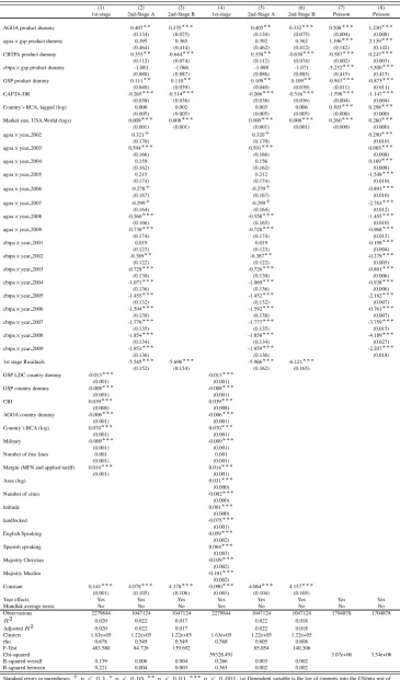
1 Summary of coefficients and impact of preference dummies . . . 24
2 Imports by the USA from SSA underAGOA . . . 32
3 Imports by the USA from SSA underGSP . . . 33
4 CBIImports by the USA, by region . . . 34
5 AGOAImports by the USA, by region . . . 35
6 Mean Imports by Applied and MFN tariffs, Selected African Countries - 1996-2009 . . . . 36
7 Mean Imports by Applied and MFN tariffs, Selected Caribbean Basin Countries - 1996-2009 37 8 Maximum Imports by Applied and MFN tariffs, Selected African Countries - 1996-2009 . 38 9 Maximum Imports by Applied and MFN tariffs, Selected Caribbean Basin Countries -1996-2009 . . . 39
Abbreviations Used
• ACP - African Caribbean and Pacific
• AGOA - African Growth and Opportunity Act
• AGOAA - African Growth and Opportunity Act Apparel waiver • ATPA - Andean Trade Preference Act
• ATPDEA - Andean Trade Promotion and Drug Eradication Act • CAFTA-DR - Dominican Republic–Central America Free Trade Area • CBERA - Caribbean Basin Economic Recovery Act
• CBI - Caribbean Basin Initiative
• CEPII - Centre d’Etudes Prospectives et d’Informations Internationales • CGE - Computable General Equilibrium
• CIF - Commission, Insurance and Freight • CUTS - Consumer Unity and Trust Society • EBA - Everything But Arms
• EPAs - Economic Partnership Agreements • EU - European Union
• FTA - Free Trade Area
• GAO - Government Accountability Office • GSP+ - Generalised System of Preferences Plus • HS - Harmonised System
• ILO - International Labour Organisation • LDCs - Least Developed Countries • LSDV - Least Squares Dummy Variable • MFN - Most Favoured Nation
• NRP - Non Reciprocal Preferences
• OECD - Organisation of Economic Cooperation and Development • OLS - Ordinary Least Squares
• ROO - Rules of Origin • SSA - Sub Saharan Africa
• UNCTAD - United Nations Conference on Trade and Development • US - United States
• USITC - United States International Trade Centre • USTR - United States Trade Representative
1
1
Introduction and Background
The United States of America (USA) has signed several preferential trade agreements with developing countries. These include theAfrican Growth and Opportunity Act (AGOA)offered to selected Sub-Saharan African countries (SSA) and theCaribbean Basin Trade Protection Act (CBTPA)which were provided to Caribbean Basin countries1. TheCBTPAis part of the earlierCaribbean Basin Initiative (CBI)which was
launched as theCaribbean Basin Economic Recovery Act (CBERA)provided to the Caribbean Basin coun-tries in the early 1980s. Although, we focus on theCBTPApreferences which were provided in 2000 we do make references to the earlierCBI andCBERApreferences. There has been much debate in the literature about the impact of these preferences for developing countries. These studies include the impact ofAGOA (for example, Brenton and Hoppe, 2006, Brenton and Ikezuki, 2004, Collier and Venables, 2007, Frazer and Van Biesebroeck, 2010, Gibbon, 2003, Mattoo et al., 2003, P´aez et al., 2010, Tadesse and Fayissa, 2008) and studies on theNorth American Free Trade Agreement (NAFTA),Caribbean Basin Initiative (CBI)and Dominican Republic–Central America Free Trade Area (CAFTA-DR)(Ames, 1993, Haar, 1990, Hornbeck,
2010, Hutchinson and Schumacher, 1994, Ozden and Sharma, 2006, Yeboah et al., 2009).
All these studies are mixed in terms of the impact of the preferences on developing countries. We believe that the mixed results can be attributed to the construction of the counter-factual by which the impact of the preferences are measured. Collier and Venables (2007), Di Rubbo and Canali (2008) and Nilsson (2005) tend to carry out their analysis by providing a means of measuring the performance of the preferential ben-eficiaries by comparing their exports to the USA to that of the European Union (EU). We envisage that this is important in isolating the impact ofAGOA given that these countries also export to other regions and also receive preferential treatment from these regions. In this paper, we instead control for the exports of the developing countries to the rest of the world. This is done in order to also control for countries that in addition to benefiting from the preferences of the US and/or the EU are also members offree trade areas within their regions and hence have intra-regional trade which are exclusive of tariffs.
Frazer and Van Biesebroeck (2010) argue that the non-uniform preferences provided byAGOAand its se-lective choice of countries from within the continent satisfy the requirement for analysing the policy impact impact ofAGOA. TheCBTPA preference was also unilaterally applied to selected Caribbean and Latin American Countries2. The variation in countries selected and products covered is employed in the analysis
to study the impact of theAGOAandCBTPApreferences on selected products at the 6 digit level of trade. Besides, Agostino et al. (2007) also notes that in the absence of these preference agreements the average level of trade becomes the counterfactual hence, adopting their idea—the introduction of theCBIandAGOA would lead to a departure from the normal level of trade. This departure from the normal level of trade can thus be interpreted as the effect of the policy.
In this paper the main question we ask is that,“has there been an observed increase in the exports of AGOA recipients to the USA compared to their exports to the rest of the world?” In addition we, (1) estimate the impact of the USA’s preferences on exports of developing countries given their exports to the rest of the world (focussing on theAGOA, CBI and GSPpreferences), (2) compare the impact at various levels of disaggregated trade (3) compareAGOAto theCBTPApreferences noting any significant differences (4)
1Caribbean and Central American Countries: Anguilla, Antigua and Barbuda, Aruba, Bahamas The, Barbados, Belize, British Virgin Islands, Cayman Islands, Costa Rica, Dominica, Dominican Republic, El Salvador, Grenada, Guatemala, Guyana, Haiti, Hon-duras, Jamaica, Montserrat, Netherlands Antilles, Nicaragua, Panama, St. Kitts and Nevis, St. Lucia, St. Vincent and the Grenadines, Suriname, Trinidad and Tobago, and Turks and Caicos Islands
determine which products have been the export drivers while comparing the importance of apparel in the exports of the preference beneficiaries and (5) show that the results are robust to the choice of econometric technique and not sensitive to controls included in the regressions. In doing this, we contribute to the exist-ing empirical literature on USA preferences by controllexist-ing for the exports of developexist-ing countries to the rest of the world. Secondly, we add to the few existing empirical work on theCBTPApreferences. In addition, we also find support for the importance of apparel and textiles inAGOA(andCBTPA) exports as has been underscored by for example Collier and Venables (2007) and Frazer and Van Biesebroeck (2010). Finally, we show that with large N panels the random effects estimator is inconsistent and inefficient. However, the Heckman two step procedure, fixed and Mundlak corrected random effects estimators provide similar estimates.
The rest of the paper is organised as follows. Section 2 provides a brief review of the empirical literature and some initial exploration of the data on preferential imports. Section 3 presents the data and methodology. Section 4 presents econometric modelling issues that need to be addressed and section 5 is a discussion of the results. The conclusion is provided in the final Section.
2
Review of the Empirical Literature
TheAGOAandCBIpreferences have undergone several amendments since their inception in 2000 (started in 2001) and 1983 respectively. We provide a summary of these important revisions in theAGOAandCBI preferences below. For theAGOApreferences the following revisions are noteworthy3:
• AGOA I - extended GSP product eligibility (4650 products); certain limitations (eg. competitive
needs legislation) removed; inclusion of 1835 products not covered in theGSPas duty free products.
• AGOA II - (2002) further relaxation of rules of origin in apparel and selected textile articles (eg.
tow-els & blankets, etc); knit-to-shape apparel included; rules of origin relaxed to include yarn; Botswana and Namibia given LDC status; volume cap limit doubled
• AGOA III - extendedAGOA to 2015 and apparel provisions to 2007, ethnic printed fabrics added;
use of foreign collars and cuffs in domestic garments allowed
• AGOA IV - (2006) Access given to LDCAGOAcountries for HS 50 - 63; new rules of origin allowing
inputs to be sourced from theAGOALDC group. Third country fabric extended to 2012; increase in volume cap on garments.
• AGOA V - (Nov. 2009) single implementation of rules of origin; harmonisation and expansion of
USA preferences and extension of trade benefits currently available.
The CBI has also undergone several phases and these include4:
• Launched in 1983 as the Caribbean Basin Economic Recovery Act (CBERA)
• 1984 - 20 countries received benefits (Includes El Salvador, Guatemala and Honduras. Nicaragua in
1990).
• 1990 - CBERA made permanent and amended.
– 20 % tariff reduction on certain leather products
3www.agoa.info andAGOAreports to congress
3
– Duty free treatment for products using 100% inputs from the US
• 1991 - 94 tariff categories added or expanded
• 1992 - 28 tariff categories added or expanded.
• 2000 - US Caribbean Basin Trade Partnership Act enacted.
– Added apparel exports
– This expires in 2010 (or if an FTA of the Americas comes into force)
• 2002 - CBERA amended
• 2006 - CAFTA-DR benefits begin for Dominican Republic, Honduras,
Guatemala, El Salvador and Nicaragua. Costa Rica joins in 2009.
• The CBTPA has however, been extended for the remaining countries beyond 2010.
2.1
AGOA
and Sub Saharan Africa
Tadesse and Fayissa (2008) use HS-2 digit disaggregated data to analyse the impact ofAGOA on exports of eligible countries to the US. In doing this they adopt a gravity model and they also separate theAGOA impact into intensive and extensive margins5. In addition to the standard gravity variables they include the
stock of immigrant population (per country) in the US, dummies for landlocked,AGOAeligibility, English language, an index of economic openness, years elapsed underAGOA, lagged imports and time and country effects. Using a tobit estimation technique they carry out regressions for each HS-2 digit product (that is chapters 00 - 99) and decompose the coefficient of the AGOA dummy into extensive and intensive margin effects.
Generally, the gravity coefficients had the expected signs—distance (-0.5) and economic size (0.495) for HS 03 products (that is fish and crustaceans). Moreover, US population and income levels had no significant impact onAGOAimports in several of the HS-2 categories.AGOAhad approximately a 64% increase in HS 03 imports although it was insignificant. The lag of the dependent variable (0.65) was significant in most of their regressions. They reported both positive and negative immigrant stocks in several cases. The ex-tensive and inex-tensive margin effects reported by them for HS 01 products were 0.085 and 0.51 respectively and significant. In relation to the decomposition, only a few products recorded significant values for both effects—much less than the 24 significant extensive margin effects across products.
Collier and Venables (2007) estimate the impact of trade preferences on exports of developing countries to the USA relative to the EU using total apparel exports. Their total sample was 110 developing and middle income countries resulting from selecting countries with mean apparel exports of US$ 100,000 and above. They capture theAGOAimpact through a dummy variable indicating when the country was givenAGOA preferences. The main regressions are also estimated for a sub sample of 86 countries whose apparel exports were US$ 1 million and above during 1991 - 2005. The coefficients forAGOAA (AGOA apparel dummy)in their first three regressions were significant and varied from 2.00 to 2.21. The coefficients signify the strong impact ofAGOAin increasing exports to the US relative to the EU in apparel products. The actual impact on exports to the US relative to the EU is given by the exponents of 2.00 and 2.21 which are 7.39 and 9.12
times the exports to the EU respectively. The result signifies an increase inAGOAcountry exports to the USA relative to the EU by a multiple of 7.39 and 9.12 respectively.
On the contrary, they had an another dummy capturing the effect of the EUEverything but Arms (EBA) preference on these countries. In order to identify the effect of theEBAthey restricted their dummy to countries that were ineligible for theEuropean Union–African Caribbean and Pacific (ACP)preferences. This variable was not significant and in most cases had the wrong sign. Similarly, using theEBAdummy in its place—it was also not significant and showed the wrong sign. Three subsequent regressions with 110 countries correct the sign for theEBAdummies and produces a marginal increase in theAGOAAcoefficient. A quadruple difference in difference method to sort out the effects of having between country characteristics vary over time is also used. In the two regressions carried out with this method, theAGOAAeffect recorded significant values (2.65 and 1.98 respectively). The first regression excluded the AGOA and EBANC terms. They therefore confirm that,AGOAhad a large impact on its beneficiaries. We depart from Collier and Ven-ables (2007) by expanding our product coverage6as well as working with highly disaggregated trade data.
Secondly, we also consider preferences offered to the Caribbean Basin countries (CBTPA). And finally, we control not only for exports to the EU but also exports to the rest of the world.
Nilsson (2005) and Di Rubbo and Canali (2008) who instead employ a gravity model do not find such strong results forAGOAin their sample. It must however, be noted that these studies did not use the same product groups and level of aggregation. Nilsson (2005) explored the effects on total exports while Di Rubbo and Canali focussed on agri-products. Collier and Venables on the other hand, limited their analysis to apparel. In summary, Nilsson (2005) and Di Rubbo and Canali (2008) did not find significant trade creating effects forAGOA. EU trade policy was found to be more trade creating compared toAGOA.
Nilsson (2005) in a study of EU and USA trade policy for 158 developing countries apply a standard gravity model in estimating the trade effects of their trade policies. Their results confirm a stronger trade creating effect of EU policy compared to the USA trade policy. However, one drawback is that, the study did not account for the zero exports in the model estimated7. This is presented as a censoring problem in the
econo-metrics literature and can create significant biases in coefficient estimates thus making them unreliable for inference (Cameron and Trivedi, 2005, Greene, 2003, Jensen et al., 2002, Wooldridge, 2002).
However, Nilsson’s (2005) cross section estimation using the 2001 - 2003 annual average exports reduce the censoring problem. The coefficients of both sets of regressions are similar; however, the t-statistics estimated in the 2001 – 2003 panel are twice the cross-section estimates indicating the potential bias of ignoring the censoring of the dependent variable in his model. The reported trade creation values for the cross-section regression8include EU imports-35.6%; low income countries-50.3%; lower middle income
countries-22.9% and upper middle income countries-46.2%. The percentages indicate the amount of trade generated by EU trade policy compared to USA policy. Thus the 50.3% reported for low income countries imply that EU policy created 50.3% more exports compared to USA policy for low income countries. All but lower middle income countries had significant coefficients in the cross-section regression. The coeffi-cients for the panel regression are not discussed in this section due to the potential bias in the coefficoeffi-cients
6We go beyond apparel products to include all six–digit products within the following categories: live animals; meat and edible meat offal; salt, sulphur, earth and stone, plastering; ores, slag and ash; and textile products.
7Nilsson (2005) in Section 4, the last paragraph of the gravity model sub-section makes reference to the zero exports–”No particular attempt is made to deal with the zero-or missing value observations in the trade data” The countries with zero or missing trade data can be found in footnote 32.
5
identified above. Finally, the average estimate of gross creation by EU policy for the period 2001 – 2003 was 70.2%, 59.3% and 54.2% of total imports by the EU from developing countries for lower income, lower middle and upper middle income countries respectively (Nilsson, 2005). This is an indication of the size of the gross trade creation by the EU trade policy.
Di Rubbo and Canali (2008) in a study of 102 developing countries for the period 1996 - 2005 for agri-cultural products (food and fibre products) use a similar methodology to that of Nilsson (2005). They find EU trade policy to be more effective at creating trade than USA policy. They report gross trade creation coefficients of 75.9%, 62.2%, 90.4% and 69.1% for low income, lower-middle income, upper-middle in-come countries and EU imports respectively for the period 1996 - 2000. Higher percentages are recorded for the period 2000 - 2005 of 80.8%, 63.1%, 91.4% and 73% for low income, lower-middle income, upper-middle income countries and EU imports respectively. A similar interpretation to Nilsson’s can be given to Di Rubbo and Canali–however, EU policy generates more exports of agri-products compared to the USA. They find the trade variation to be significant for the lower income group. Compared to Nilsson (2005) the trade creation effects are stronger for the upper-middle income countries rather than the low-income countries. We note that, these effects are confined to the agri-food sector not total exports as was the case in Nilsson. Also, the reported coefficients of Nilsson above, are for his cross-section regression and therefore exclude the time variation provided by Di Rubbo and Canali (2008).
In similar fashion, a recent paper by Frazer and Van Biesebroeck (2010) estimates the impact ofAGOAat the HS 8 - digit level using standard difference-in-differences and triple difference-in-differences – control-ling for baseline levels of imports, country and product specific import trends after the adoption ofAGOA. They find an increase of 42% of imports on average as a result of theAGOApreference. However, they estimate the causal impact ofAGOAto be lower at 28%—they argue that this controls for both the pre- and post-import differences for bothAGOA and nonAGOAcountries—as well as control for product-specific trends common for both groups of countries. On the contrary, concentrating on only non-oil imports they find the increase to be 6.6%.
In summarising, Collier and Venables (2007), Frazer and Van Biesebroeck (2010), Gibbon (2003), P´aez et al. (2010) generally find apparel and textiles as well as oil and energy products to be the main drivers of the gains byAGOAbeneficiaries. We do observe this also in our analysis and it is further discussed in Section 5. Gibbon (2003) and P´aez et al. (2010) discuss the proliferation of firms in the textile industry and the enormous impact on employment in that sector for Lesotho and other African countries. This according to them is not limited to apparel but also to oil and energy related exports where the example provided is the increase in investments in Nigeria’s energy sector. Nonetheless, for Lesotho in spite of the record investments an impediment in having further investments was the constraints on land available (Gibbon, 2003). Had these constraints not existed a much stronger impact ofAGOAmight have ensued.
In an extended survey of previous empirical studies, Mold (2005) links the mild impact ofAGOAto (1) the limited benefits and exclusion of sensitive products from theAGOAlist, (2) the initial 8-year life span of AGOAwith the subsequent extension in 2004 (ofAGOA) to 2015 has not encouraged long-term investments
periodic (annual) review ofAGOAbeneficiaries.
2.2
CBI
and Caribbean Basin Countries
TheCBERApreferences were less effective than theCBTPApreferences (Hornbeck, 2010) and this shows in the jump we observe in Figure (4(a)) in Appendix I. However, this is explained by Hutchinson and Schu-macher (1994) to be as a result of (a) over-reliance on the market mechanism, (b) the exclusion of important Caribbean Basin products such as textile and apparel as well as tourism products hindered the reaping of its potential benefits, (c) the re-imposition and tightening of US sugar quotas and (d) the falling world prices of petroleum and petroleum products. This has led many authors to conclude thatCBERApreferences failed to achieve their mandate of increasing economic growth in the region (for example, Ames, 1993, Hornbeck, 2010, Hutchinson and Schumacher, 1994). Nonetheless, theCBTPApreferences which had a large impact on the recipients also met with a decline as a result of the introduction of theCAFTA-DR(this is observed as the declining trend for our selected Caribbean countries in Figure (4(a))).
Hornbeck (2010) argues that CBI beneficiaries have suffered from erosion of their preferences as a result of the increasing move towards the adoption offree trade agreements (FTA)by the USA.NAFTAafter its adoption, curtailed the trade advantage of theCBI countries over Mexico—thereby giving Mexico some advantages in apparel and other products Mexico was more competitive at producing than the Caribbean Basin countries (Hornbeck, 2010, Hutchinson and Schumacher, 1994). Hutchinson and Schumacher (1994) in calculating the revealed comparative advantage (RCA) of Mexico and the Caribbean countries in their top 30 export products did find the Caribbean countries to be competitive in 20 out of their top 30 industries and expected this to provide some buffer againstNAFTA. The adoption of theCAFTA-DRhas in particular adversely affected the remaining Caribbean countries within theCBIand again reduced their trade advan-tage in apparel and textiles and non-primary commodities (Hornbeck, 2010). The main reason provided by Hornbeck (2010) is due to the cummulation rules in apparel production amongNAFTA, CAFTA-DRand Haiti which leave the remaining countries under theCBIwith limited ability to adapt to the new competition from these regions. The percent of apparel imports in total US imports of apparel is even lower–this fell from 13.6% in 2005 to 1% in 2008 (Hornbeck, 2010). Hornbeck (2010) attributes this to theCAFTA-DR — CAFTA-DRcountries excluding Costa Rica accounted for 90% of total apparel imports of all the Caribbean Basin countries (Hornbeck, 2010) and this accounts for the vast shortfall.
Hornbeck (2010) shows that only 7.5% of total imports fromCBI recipient countries were eligible for preferential tariffs after excludingCAFTA-DRand energy exporting countries. This is what might be driving our negative coefficients discussed in section 4 of this paper. In addition, Hornbeck (2010) finds that the following additional factors contributed to the diminishing preferences (a)CAFTA-DRcountries produced most of the apparel and textile products (b) the remainingCBIcountries are not competitive in the apparel sector and have been unable to take advantage of the preferences and (c) The removal of themultifibre agreement (MFA)on textiles has furthered heightened their situation. It must however, be added that some
7
2.3
Trends in Imports to the USA from Selected
AGOA
and
CBI
beneficiaries
The variation in the exports under the various programmes are shown in the graphs at the end of the paper in Appendix I. Figures (2) and (3) show the relationship between the preferential exports and mean aggregate exports (1997-1999) to the USA forAGOAandGSP. Figures (4) and (5) on the other hand, show the trends in the share of preferential exports in aggregate preferences and total exports to the USA respectively. For theGSP preference South Africa is the main outlier while Nigeria is the outlier forAGOAexports. Ex-cluding these two countries in Figures (2(a)) and (3(c)) for those with exports greater than the mean total exports for the period 1997-1999 ($35.37 million) improves the fit and the line becomes steeper (Angola now becomes the outlier with exports close to $1 billion) to the USA.
There is no clear indication of the relationship for countries below the mean, however, rescaling the the graph would show a very steep line of fit as in (3(c)) for these countries. In Figure (4), the selected CBI countries within Latin America in (4(b)) do not show much difference between their shares. On the con-trary, a clear jump in the share of exports for the selectedAGOAcountries in (5) is noticed in 2001 (countries begin to use theirAGOApreferences). Similarly, noticeable differences exist in (4(a)) with the prominent case being the large jump in 2005 for Barbados but which gradually falls over time.
Figures (6) and (7) show the mean imports by applied and MFN tariffs for selected African and Caribbean Basin countries at the 6 digit level. Figures (8) and (9) show the maximum imports into the USA within each category. Ghana and Barbados are observed to export under each category. However, their mean im-ports into the USA are far below US$1 million and that of the remaining countries (with the exception of Angola that has mean imports into USA below US$ 20000). Kenya, Costa Rica and Jamaica have higher means, however, these are concentrated in two dominant categories—apparel and textiles, and salt/ore, slag and Ash exports. For the selectedAGOAbeneficiaries, their mean imports into the USA are dominated by free imports. The same can be said of Barbados and Jamaica. Although Ghana had low mean imports into the USA of apparel, the maximum imports into the USA from Ghana are concentrated in apparel and the imports are above US$ 6 million. For the remaining countries the pattern in the mean category is maintained.
3
Data and Methods
Data for the analysis is obtained from the World Integrated System9(WITS) which queries data from UN
Comtrade for export (and import) data and UN TRAINS for the tariff data. Gross domestic product data is obtained from The World Bank’s World Development Indicators10 (WDI) and gravity type variables (viz., landlocked, area, latitude, number of cities, official language, etc) are obtained from the CEPII distances database11. In addition, our political variables (military and religion) are obtained from the Database of
Political Institutions12 (DPI) and democracy time series dataset13. Finally, the preferential dummies are
constructed based on information sourced from the WITS preferential database and USITC14The
remain-ing variables constructed (viz., RCA and market size) are based on the variables obtained from the sources above. Table (1) provides further information on the variables used as well as summary statistics.
We selected HS 2-digit categories 01:- Live Animals, 02:- Meat and edible meat offal; 25:- Salt, sulphur, earth & stone, plastering, etc; 26:- Ores, slag and ash; and 50–63:- Apparel and clothing and then used all the 6-digit categories within these 2-digit choices. The products were selected based on whether some of the 6-digit products were captured in the preference. Also, of interest were products that form a signifi-cant component of developing country exports. Apparel and Textiles are an important component of both AGOAandCBTPApreferences hence their inclusion. Arguably, agricultural produce and energy and energy
related products are important in the exports of some of the beneficiary countries, however, we excluded these products from our analysis given that majority of the countries offered these preferences are net oil importers. Secondly, energy products form a significant component of AGOA exports to the USA—we therefore seek to carry out the analysis excluding these products to see if a positive impact is still observed.
We use annual data covering the period 1996 – 2009. There are 166 countries and 981 different products at the 6 digit level in the dataset. The products comprise of 808 apparel and textile and 173 non apparel and textile products at the 6-digits level. Fewer products are however, exported by several of the countries. For example, for the African countries fewer than 400 products are exported in any given year. Of these products there are some products that are not exported in all years. In Table (1), the probability of exporting a particular 6-digit product in our sample is 0.342, the average number of free lines per 6-digit category is 0.444, the average weighted MFN tariff is 9.03% and the average applied tariff is 8.09%. The probability of exporting under theGSP, AGOA, CAFTA-DRandCBTPAare 0.008, 0.004, 0.01 and 0.007 respectively. The tariff margins are constructed based on information provided at the 6-digit level on the MFN and applied tariff provided by WITS. In cases where missing values are encountered we checked the preferential status of the country and replaced the missing values with the average estimate based on the region, preference group and product. Exports not provided by UN Comtrade were assumed to be zero. This holds since for developing countries we use mirror exports (that is, the USA and World import values from these countries) in place of the actual export values. By doing this, we are able to observe whether they actually exported those products. Nonetheless, the mirror export values are better recorded than the export values from the developing countries (Piermartini and Teh, 2005).
9http://wits.worldbank.org/wits/ 10http://data.worldbank.org/
11Centre d’Etudes Prospectives et d’Informations Internationales: http://www.cepii.fr/anglaisgraph/bdd/distances.htm
12Thorsten Beck, George Clarke, Alberto Groff, Philip Keefer, and Patrick Walsh, 2001. ”New tools in comparative political economy: The Database of Political Institutions.” 15:1, 165-176 (September), World Bank Economic Review.
9
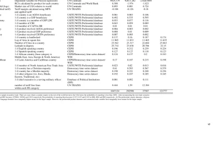
Table 1: Variable definitions and summary statistics: 1996 – 2009
Variable Name Variable Description Source HS6-Mean HS4-Mean HS2-Mean Time invariant (at HS6)-Mean Probability of exporting Dependent variable for 1st stage of Heckman. UN Comtrade 0.342 0.282 0.16
1 if country exports to the USA
US/World Import ratio (logs) Dependent variable for all other regressions UN Comtrade 0.323 0.293 0.202 US/World Import ratio Dependent variable for Poisson regressions UN Comtrade 9824.379 92813.282 -2.82E+004 Country’s RCA (log) RCA calculated by product for each country UN Comtrade and World Bank 0.588 -1.974 -1.821 Market size, USA.World (logs) Market size of USA relative to world UN Comtrade 0.895 0.881 0.724 Margin (MFN and applied tariff) Tariff margin calculated using MFN UN TRAINS -0.108 -0.126 -0.18
and applied tariff
AGOA country dummy 1 if country is an AGOA beneficiary USITC/WITS Preferential database 0.061 0.083 0.106 GSP country dummy 1 if country is a GSP beneficiary USITC/WITS Preferential database 0.492 0.535 0.595 GSP LDC country dummy 1 if country is a member of GSP LDC USITC/WITS Preferential database 0.053 0.077 0.116 CBI 1 if member of CBI USITC/WITS Preferential database 0.043 0.059 0.089 CAFTA-DR 1 if member of CAFTA-DR USITC/WITS Preferential database 0.01 0.01 0.01 AGOA product dummy 1 if product received AGOA preference USITC/WITS Preferential database 0.004 0.003 0.002 GSP product dummy 1 if product received GSP preference USITC/WITS Preferential database 0.008 0.01 0.009 CBTPA product dummy 1 if product received CBTPA preference USITC/WITS Preferential database 0.007 0.005 0.002
landlocked 1 if country is landlocked CEPII 0.137 0.16 0.187 0.174 Area (log) Log of Area in square km CEPII 11.965 11.833 11.465 11.635 Number of cities Number of Cities in a country CEPII 23.542 23.317 22.684 23.043
latitude Latitude in degrees CEPII 25.734 23.638 20.786 22.15
English Speaking 1 if English speaking country CEPII 0.196 0.212 0.239 0.224 Spanish speaking 1 if Spanish speaking country CEPII 0.127 0.127 0.118 0.123 Africa 1 if African country (base category is CEPII/Democracy time series dataset/ 0.124 0.157 0.2 0.183
Middle East, Asia, Europe & North America) WDI
Latin America & Caribbean 1 if Latin America and Caribbean country CEPII/Democracy time series dataset/ 0.17 0.187 0.215 0.198 WDI
NAFTA 1 if member of North American Free Trade Area USITC/WITS Preferential database 0.023 0.02 0.013 0.016 Majority Christian 1 if country has a Christian majority Democracy time series dataset 0.61 0.593 0.567 0.579 Majority Muslim 1 if country has a Muslim majority Democracy time series dataset 0.198 0.221 0.248 0.236 Other religion (base) 1 if other religion (viz, Jews, Hindu, Democracy time series dataset 0.192 0.187 0.185 0.185
Eastern, Traditional, etc)
Military 1 if chief executive is a serving military officer Database of Political Institutions 0.081 0.092 0.111 (DPI)
Number of free lines number of tariff free lines UN TRAINS 0.444 1.59 12.384 within each HS category
Observations 1047124 292598 37567 121777
Finally, it is acknowledged that the tariff margin variable might be measured with some error given the paucity of tariff data available on UN TRAINS. We do, however, believe that this would not seriously affect our estimates presented in the results section. As a result, the tariff margin is not used in all regressions—in its place, we allow the country-product fixed effects to capture the tariff margin. Doing this makes it possi-ble to check if the coefficients are biased in the absence of the tariff margin as an additional regressor.
The econometric formulation for investigating trade preferences at the macro level is adopted from Collier and Venables’s (2007) paper. They estimate the impact of the USA’sAGOAand EU trade preferences (given by dummies) on the log of exports from developing countries to the USA relative to the EU-15 countries. They control for market size and market demand shocks. We depart from Collier and Venables (2007) by looking at disaggregated 6 digit HS chapters 1, 2, 25, 26 and 50-6315 and instead use the ratio of imports
by the USA relative to imports by rest of the world for each country (see equation 4). Additional controls included here are each countriesRCA, lagged values of applied preferential and MFN tariffs (or preference margins) at the 6-digit product level and lagged political controls such as democracy and political stability. In addition, imports under the GSP is controlled for by interacting our GSP dummy with theCBIandAGOA dummies.
At the 6 digit level of disaggregation, zero exports would be observed for some countries hence the Heck-man two-stage panel estimator is more appropriate in modelling Equation (5). This is needed to correct for selectivity bias in the decision to export a particular HS 6 digit product in the case of the Heckman selec-tion. Essentially, there is self-selection in the exports of products at highly disaggregated levels, whereby countries do not randomly choose to export a particular product. Our panel approach to estimation allows us to include fixed effects (exporter and product fixed effects) and time effects to control for some of the unobserved characteristics and market shocks respectively. The principal model is the Heckman selection — the Poisson pseudo maximum likelihood estimator (PPMLE), panel fixed effects, and Mundlak corrected random effects models are included for comparative purposes.
Equation (1) and (2) below model exports from country i (partner) to j (USA) and rest of the world as a function of exporter nation characteristics (E), USA and World characteristics - captured by market size (M), between country characteristics (d) and an error term (µ). The total imports by the USA relative to the World of productpfrom all countries is the proxy for market size–which additionally controls for market demand shocks in these importing regions. The between country characteristics (d) includes fixed elements-for example distance and constant trade preferences over time as well as time varying country-pair specific trade preferences (Collier and Venables, 2007, 1338-9). We proxy these using exporter and product fixed effects for the constant parts and dummies for trade preferences for the time varying parts. Equation (3) is then the ratio of the first two equations–this substitutes out the exporter characteristics leaving us with an estimable equation in the form of Equation (5). Equation (4) is our selection equation and theInverse Mills Ratiocalculated from (4) is incorporated into (5) to complete the Heckman two-step procedure.
The PPMLE is estimated using Equation (3) in its multiplicative form. The Poisson regression log linearises this equation and thus our results would be similar to the log linearised model in Equation (5) (for example, Herrera, 2010, Silva and Tenreyro, 2003). Our argument is that a country given a preference would then decide which products to produce. In this decision, rules of origin, cummulation rules, preference margins, competitiveness and other factors determine whether the country exports to the USA. In modelling the
11
ond stage we do not believe that, the preference margin then plays a significant role since this is captured in the product exported under the preference. Hence our exclusion restriction includes the preference margin and this is discussed further in the next section.
Xip,j=Ei(t)∗Mj(t)∗dip,j(t)∗µip,j(t) (1)
Xip,w=Ei(t)∗Mw(t)∗dip,w(t)∗µip,w(t) (2)
xipt=Mt∗dipt∗µipt (3)
exportsipt=α+β′T Pit+γ1lat+γ2RCAi,wipt +γ3M ilipt−1
γ4tarif f marginipt−1+ Γ′Za+ηip+ηt+µipt (4)
exportsipt=
1 if positive exports
0 otherwise
lnxipt=a+α′T Pipt+γ1M Sizept+γ2RCAi,wipt−1+
+ˆλipt+δ′Zb+ηip+ηt+ǫipt. (5)
Where:xipt= XXip,wip,j;Mt= MMwj;dipt=ddip,wip,j
i, p, and tsubscripts refer to country, product and time respectively, jrefers to the USA whilewrefers to rest of the world,“a”in Equation (5)
is the constant of the regression. The log of the dependent variable is taken asln(1 +X). Tariffs and political variables are lagged in order to avoid
introducing any simultaneity or endogeneity into our model.
Xij is Imports from partneri
Ei is exporter nation characteristics
Mj is importer characteristics
dij is between country characteristics - given by trade preferences offered byjtoi
µipt;ǫipt is an error term
T Pit is trade preferences offered by the USA. It takes the value 1 from the year in which a country first receives
the preference and 0 before16. Includes, GSP, AGOA and CBI beneficiaries
T Pipt is trade preferences offered by the USA. It takes the value 1 for a product exported under a preference and
0 otherwise17. Includes, GSP, AGOA and CBTPA beneficiaries for each product
M Sizept is market size the ratio of total imports of our selected commodities intojexcluding countryi.
tarif f marginipt calculated asM F N tarif fM F N tarif f−Applied HS tarif ffor each country, year and product.
M il is Military - 1 if chief executive is a serving military officer
ˆ
λipt Is the inverse Mills ratio from the first stage regression, calculated as: φΦ((··)),
whereφ(·)is the standard normal probability density function andΦ(·)is the standard normal density function of the Equation (4) whenE(exports= 1|covariates).
ηt Time effects
ηip exporter and product fixed effects in the fixed effects regression. Is the random effects in the panel random
effect models Za
vector of control variables – latitude, natural log of area, number of cities, Number of Free lines, dummies for Africa, Latin America & Caribbean, landlocked Christians, Muslims, English and Spanish speaking countries
Zb vector of control variables – latitude, natural log of area, number of cities, dummies for landlocked, Africa,
Latin America & Caribbean,NAFTA, CAFTA, English and Spanish speaking countries RCA Based on Balassa (1967)18the revealed comparative advantage (RCA) is calculated as:
RCAi,wipt=
Xwp,i
P
pXwp,i
÷
Xwp,w
P
pXwp,w
where: Xw
p,iis exports of productpfrom countryito the World and
P
pX w
p,iis total exports from
countryito World,Xw p,wand
P
pX w
p,ware the world exports of productpand total exports respectively
16Definition allows preferences to overlap for each country. Thus a country can be anAGOAand aGSPbeneficiary. To control for these overlaps we include interaction terms for those cases where countries have two or more preferences
17Previous footnote applies here also
4
Econometric Modelling Issues
We attempt various econometric techniquesviz., the Heckman selection and the Poisson models. These are then compared to traditional estimates from the fixed effects and random effects models based on positive export flows. We employ the fixed effects regressions in most of our estimations as this approach allows for the existence of a correlation between the fixed effects and the regressors (Baltagi, 2001, Greene, 2003, Wooldridge, 2002). Secondly, the fixed effects approach minimises the omitted variable problem as the fixed effects capture variables omitted from the model leaving the coefficients unbiased to a large extent. A problem with the fixed effects is the inability to estimate time invariant variables. However, the time invariant variables can be recovered from a regression of the variables on the extracted fixed effects. The time invariant variables are not pivotal to our analysis so this is pursued only in a couple of regressions for comparison purposes—that is to compare the coefficients to those of the random effects, which allows for time invariant variables.
Unlike the fixed effects, the random effects approach does not allow for a correlation between the random effects and the explanatory variables. The model assumes this correlation to be zero. Hence, in the presence of a correlation, the random effects model becomes inconsistent and inefficient. Additionally, Mundlak (1978) argues that the random effects model in the presence of the correlation is misspecified. Mundlak (1978) argues that the random effects model is biased when there is a correlation between the random effects and the explanatory variables. To overcome this, Mundlak (1978) suggests adding the mean of the explanatory variables as additional regressors in the random effects model. Thus in our case theηip in
Equation (4) and (5) (when estimated by random effects can be assumed to be capturing the random effects) can be specified as:
ηip =ϕ′X¯ip+ϑip (6)
where:
ϑip∼N(0, σϑ2), X¯ip =
PT t=1Xipt
T and X is the vector of explanatory variables in Equation (4) or (5)
This is pursued for all the random effects models presented in the results section. TheHausman testallows a choice to be made between the fixed effects and the random effects models. In addition, theBreusch and Pagan testprovides a way of testing whether the random effects are significant. In Table (2) we report the
Breusch and Pagan testand these are significant for all random effects models estimated (with and without
Mundlak’s correction). TheHausman testis not pursued since we employ the fixed effects model to capture country and product specific effects that are not captured by the variables included in our model. The fixed effects are significantly different from zero in all estimations as provided in the table’s footnotes.
13
PPMLE. The Heckman selection is motivated by the desire to model the self-selection into export markets (for example, Agostino et al., 2007, Cardamone, 2007).
It was earlier mentioned that, mirror exports are used to help reduce the missing or unrecorded exports of developing countries. The missing data problem is not entirely resolved as this is symptomatic of highly disaggregated trade data. However, we are reassured of the reliability of the import data since import data tend to be more accurately recorded compared to export data (for example, Piermartini and Teh, 2005). This is the case since tariffs have to be applied to imports at the border. Thus, in our case, imports into the USA would be more reliable since the USA has to decide which imports are allowed in duty free, under the various preferences, MFN or at normal tariff rates—this makes them more reliable. One can safely conclude that most of the remaining missing or unrecorded values in the dataset represent countries not exporting that particular product. This essentially motivates the Heckman’s two stage panel estimator to control for self-selection into export markets and thus reduce the problem of selection bias that arises.
Import data includes cost insurance and freight charges. This is absent in export data that is reported free on board (Piermartini and Teh, 2005). In addition, this creates an estimation problem due to the correlation between imports and the error term as a result of transport costs (Piermartini and Teh, 2005). We do not expect this to pose any problems since we take the log ratio of mirror exports from developing countries to the rest of the world as the dependent variable. The use of this ratio cancels the transport costs and some constant characteristics of the exporters from the model.
An issue prevalent in pursuing Heckman’s selection model is finding appropriate exclusion restrictions. The use of appropriate exclusion restrictions reduces the bias in standard errors calculated at the second stage and allows the model to be identified (Bushway et al., 2007). Nonetheless, the use of a probit in the first stage without the necessary exclusion restrictions holds as the non linear nature of the probit model pro-vides identification (Zabel, 1992). In circumstances where both the first stage and the second stage are non linear (or linear if the first stage is based on a linear probability model) then the exclusion restrictions are important in identifying the second stage (Zabel, 1992). More importantly, failure to find adequate exclu-sion restrictions implies that the second stage cannot be identified in this case and estimates of the second stage would be inconsistent and inefficient (Zabel, 1992). To overcome these issues we adopt Jensen et al.’s (2002) approach of estimating a Mundlak corrected random effects probit model in the first stage and a fixed effects model in the second stage. This reduces the problem of having omitted variables in the first stage as well as mis-specifying the model. The challenge in carrying out the first stage probit model in our case is getting the model to converge—especially for the disaggregated product regressions. If faced with this problem we can safely adopt a linear fixed effects or a Mundlak corrected linear random effects estimator for the first stage. This, then requires us to include valid restrictions in our first stage to aid the identification of our second stage regressions.
sec-ond stage, the tariff margin serves as an exclusion restriction. After a country has decided on exporting, the tariff margin then has a lesser emphasis in encouraging exports since other factors such as competitiveness and capacity of the country becme more important. In our analysis, the tariff margin would be captured by the product dummies19 at the second stage and in the other regressions as well as the country-product fixed effects. The dummy-time interactions in later regressions capture annual variations and modifications occurring within the preference programmes.
The PPMLE has been shown to provide consistent results for gravity models and in our case it would also yield consistent estimates. Thezero inflated poisson (ZIP)model can be an alternative to the PPMLE since it models excess zeros through a logit and hence solves any headaches with selection20. However, this is not pursued due to estimation problems encountered—due to the large number of parameters (mainly the fixed effects) the model is unable to converge. Another model within thepseudo maximum likelihoodfamily, thenegative binomial regression (NBREG)is also a useful alternative in the presence of over-dispersion in the dependent variable. However, the NBREG is sensitive to the scaling of the dependent variable and is restrictive. It does not do well in the presence of excess zeros, thus it is not pursued here. Bosquet and Boulhol (2010) show that the NBREG PMLE is not consistent and is sensitive to the scale of the dependent variable—thus not good for modelling trade flows. On the contrary, the PPMLE is consistent as long as the conditional mean function is correctly specified (Cameron and Trivedi, 1998). As a result the PPMLE can be applied to data generating processes for the dependent variable in cases where it is not poisson dis-tributed (ibid.).
Finally, Piermartini and Teh (2005) argue that GDP is unreliable in estimations using disaggregated data and that the right controls in such cases is output data for the exporting industry or sectoral-country specific effects. In this paper, product-country effects are included in all fixed effects estimations and an additional variable, the revealed comparative advantage for each country is included to capture its competitiveness at the product level. This hopefully, solves the problem and reduces any omitted variables problem from not controlling explicitly for sectoral output.
5
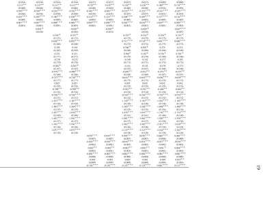
Results and Discussion
The results in this section focus on the HS-6 digit level of disaggregation. All regressions apart from the regression of time invariant characteristics on the fixed effects in Table (4), include country-product and time fixed effects. All regressions with the exception of the random effects probit and thePoisson PMLE fixed effects estimates report robust standard errors clustered around the country-product groups. Table (2) reports three different estimators—the fixed, Mundlak corrected random effects and the ordinary panel random effects estimators. Table (3) reports the Heckman two-step estimator and the Poisson PMLE. This allows allows a comparison of the various estimators and also to show any indication of bias in our chosen Heckman model. Table (4) presents the time invariant variables regressed on the extracted fixed effects reported in the first four columns of Table (2) and the Heckman second stage estimations in Table (3). Fi-nally, Table (5) allows us to check the sensitivity of our estimates to the exclusion of OECD and European countries as well as China and Hong Kong from our regressions. In Appendix II, more results are presented showing estimates of other levels of disaggregation (HS2 and HS4)—to show whether our estimates are sensitive to the level of disaggregation. Additionally, the tables in the appendix also compare estimates of non apparel and textiles to those of apparel and textiles to confirm whether the USA preferences are being
15
driven by apparel and textiles.
We next discuss the results in the main paper. Columns (1) - (4) of Table (2) reports estimates from the fixed effects regression. The difference between columns (1) and (2) is the inclusion of the military variable in column (2). Columns (3) and (4) augment Columns (1) and (2) respectively with the interaction ofAGOA andCBTPApreferences with year dummies respectively. The base year for theAGOA-year interaction is 2001 and that for theCBTPA-year interaction is 2000. Thus these two interaction terms are dropped from the regression and become the reference categories in interpreting the remaining preference-year interac-tions in the regression. Columns (5) - (8) reports the Mundlak corrected random effects—these follow the same pattern as columns (1) - (4). The main difference is the incorporation of time invariant variables. Thus in column (6) and (8) dummies for Christians and Muslims (base category is other religions) are included in addition to military. The inclusion of military and the religious dummies in these models allows us to test whether they can be omitted from the model and used as valid exclusion restrictions for the Heckman two-step estimator. We can reject the alternate hypothesis that the military coefficient is different from zero at the 5% level of significance in columns (2), (4), (6) and (8)—thereby indicating that it is not correlated with the dependent variable in the second stage. We cannot do the same for the religious dummies which are significantly different from zero at the 0.1% level and thus correlated with our dependent variable. Hence, if used in the Heckman first stage as an exclusion restriction, the residuals might be correlated with the second stage error. The Muslim dummy is however, not significant at conventional levels in columns (4) and (8) of Table (4) when regressed on the fixed effects. The final two columns of Table (2) reports the ordinary random effects estimator.
TheAGOA, CBTPAandGSPpreferences are significant in all eight columns of Table (2). Our controls CAFTA-DR, the lag of each country’s RCA and market size of the USA are also significant in all columns.
The interaction ofGSPandAGOAis not significant in any of the columns of the table. The interaction ofCBTPAandGSPis however, significant in our random effects type models. With the exception of the English speaking dummy all other time invariant controls included in the random effects type models are significantly different from zero. NAFTAhas a coefficient of 1.7 in the Mundlak corrected random effects models indicating thatNAFTAincreases exports to the USA relative to the world by 447.39% compared to nonNAFTAcountries. Similarly, Latin American and Caribbean countries on average and holding all things constant significantly increase exports to the USA relative to the world. These are expected given the close proximity ofNAFTAcountries and to a large extent the Latin American and Caribbean countries to the USA. On the contrary, on average and holding all else constant, African exports to the USA are significantly lower relative to the rest of the world in the Mundlak regressions but positive in columns (9) and (10). In sum-marising, Table (2) indicates thatAGOAandGSPpreferences increase exports to the USA relative to the rest of the world holding all else constant. WhileCAFTA-DRdecreases exports to the USA relative to the world.
Turning our attention to the next table (Table (3)) we find qualitatively similar results.AGOAis positive and significant in both the Heckman model and thePoisson PMLE. Similarly, theCBTPApreferences are only positive when the annual variation to the preference is controlled for. On the contrary, theGSPbecomes negative in thePoissonmodels. They are however, significant in all models in which they appear within the table. In both tables the annual variation of theAGOApreferences indicates that the first few year of AGOAsaw a rapid rise in exports to the USA relative to the rest of the world compared to the base year
of 2001. Columns (1) and (4) report the first stage results for our Heckman model. All variables with the exception of the number of free lines have a significant impact on the probability of exporting to the USA. Apart from countries that qualify for theCBI, all the remaining preferences, that is,GSPandAGOAeligible countries significantly lower the probability of exporting to the USA. A country’s competitiveness (RCA) in a product and the tariff margin significantly increases their probability of exporting to the USA. This is in line with our earlier assertion in the preceding section that, the larger the margin between theMFN tariff and the applied tariff (in this case the preferential tariff) the more likely a country would try to exploit the gains from exporting that particular product. Nonetheless to exploit these advantages a country with a competitive advantage in production of productpis more likely to benefit from the higher tariff margins by increasing its exports.
In column (4), latitude, English and Spanish speaking as well as land area significantly increase the probabil-ity of exporting to the USA holding all else constant. The remaining variables, number of cities, landlocked, Christianity and Muslim dummies (compared to the other religions) reduce the probability of exporting to the USA. The negative coefficients for the Muslim and Christian dummies might largely be due to the Chi-nese effect. However, for the Muslim dummy the composition of the exports of Muslim countries is also playing a role here. The military coefficient significantly lowers the probability of exporting to the USA. This is evidenced in the fact that, the USA normally imposes trade sanctions on countries it believes to be undemocratic or ruled by military leaders. The significance of military and the religious dummies indicate that they must be included in the first stage regression. They are thus highly correlated with the probability of exporting to the USA. In addition, all exclusion restrictions are jointly significantly different from zero. The case for military is however, much stronger than the religious dummies. The main difference between the two first stage regressions is that column (1) is based on a fixed effects regression, while column (4) is a Mundlak corrected random effects estimator—modified from that proposed by Jensen et al. (2002). Col-umn (4) allows additional exclusion restrictions in the form of the religious dummies as well as additional controls provided by the time invariant variables.
17
the standard errors are unbiased. This result can be attributed to the large sample dimension of our data and given that our estimators have large N and small T sample properties we can overlook the correction at this stage.
Given these comparisons, all models presented with the exception of the ordinary random effects estimator are consistent to a large extent. The ordinary random effects model however, has presented us with rela-tively larger coefficients—at times twice the estimated coefficients in the other models. This points to its inconsistency and inefficiency, hence the other models perform better in reducing this bias. An argument which we do not find tenable here is whether the model is misspecified and that the random effects model is inappropriate. It does not seem so, since the Mundlak corrected random effects attenuates the bias of the ordinary random effects. The explanation could be the presence of a correlation between the random effects and some explanatory variables. Thus the inclusion of the averages of the explanatory variables as suggested by Mundlak (1978) has greatly reduced the misspecification and problems created by the as-sumption of no correlation. Nevertheless, theρreported by the random effects type models is significantly different from zero indicating that the random effects model is preferred to a pooled OLS regression. In addition, the Breusch and Pagan LM tests of random effects indicate the presence of the random effects and these are significantly different from zero. Finally, the goodness of fit measures of the Mundlak cor-rected random effects are larger than those of the ordinary random and fixed effects models. As a result, the Mundlak random effects model provides a better fit and is the more appropriate model to present.
Table (4) shows the median and OLS regression of the time invariant variables on the fixed effects. Apart from theNAFTAcoefficient the median regressions report lower coefficients compared to the OLS regres-sion. In almost all cases there are no sign reversals. Comparing the coefficients to that of the Mundlak corrected random effects model, it is observed that Spanish speaking, English speaking and African dum-mies are now positive in the fixed effects models. TheNAFTAcoefficient is smaller than that reported in Table (2). The first eight columns of Table (4) correspond to the first four columns of Table (2). The remaining four columns correspond to the Heckman second stage regression in Table (3). To sum up, the remaining coefficients have the same sign as the random effects models but are marginally larger in most cases.
The final table reports results for a sub-sample of countries. In columns (1), (3) and (4) we exclude OECD and European countries from our sample leaving us with 119 countries. In columns (2), (5) and (6) China and Hong Kong are also excluded in addition to the countries excluded earlier. These provide us with fur-ther sensitivity and robustness checks. In addition, we want to show whefur-ther in the absence of China (which is competitive in similar products) theAGOAandCBTPApreferences show larger and more significant co-efficients. The results are qualitatively similar to the ones reported earlier. The only difference is in the first stage regression, the GSP eligible country dummy is now positive. Indicating that in the presence of the more competitive OECD countries and China, there is a marginally higher probability of exporting under theGSP.
19
Table 2: Fixed/Random effects regression without selection correction
(1) (2) (3) (4) (5) (6) (7) (8) (9) (10) FE1 FE2 FE3 FE4 Mundlak1 Mundlak2 Mundlak3 Mundlak4 RE1 RE2 AGOA product dummy 0.324∗∗∗ 0.324∗∗∗ 0.384∗∗ 0.385∗∗ 0.456∗∗∗ 0.456∗∗∗ 0.417∗∗ 0.417∗∗ 0.818∗∗∗ 0.825∗∗∗
(0.076) (0.076) (0.135) (0.135) (0.076) (0.076) (0.136) (0.136) (0.140) (0.140) agoa×gsp product dummy 0.398 0.397 0.429 0.428 -0.013 -0.014 0.025 0.024 -0.074 -0.072 (0.426) (0.426) (0.477) (0.478) (0.523) (0.523) (0.565) (0.565) (0.539) (0.541) CBTPA product dummy -0.670∗∗∗ -0.670∗∗∗ 0.367∗∗ 0.368∗∗ -0.653∗∗∗ -0.653∗∗∗ 0.394∗∗∗ 0.395∗∗∗ 1.218∗∗∗ 1.216∗∗∗
(0.075) (0.075) (0.113) (0.113) (0.075) (0.075) (0.113) (0.113) (0.111) (0.111) cbtpa×gsp product dummy -1.098 -1.098 -1.115 -1.115 -1.548∗ -1.548∗ -1.559∗ -1.559∗ -1.219∗ -1.218∗ (0.914) (0.914) (0.914) (0.914) (0.617) (0.617) (0.617) (0.617) (0.600) (0.600) GSP product dummy 0.113∗∗ 0.113∗∗ 0.113∗∗ 0.113∗∗ 0.125∗∗ 0.125∗∗ 0.126∗∗ 0.126∗∗ 0.180∗∗∗ 0.176∗∗∗
(0.040) (0.040) (0.040) (0.040) (0.040) (0.040) (0.040) (0.040) (0.034) (0.034) CAFTA-DR -0.505∗∗∗ -0.505∗∗∗ -0.242∗∗∗ -0.243∗∗∗ -0.483∗∗∗ -0.483∗∗∗ -0.222∗∗∗ -0.222∗∗∗ -0.141∗∗∗ -0.145∗∗∗
(0.036) (0.036) (0.038) (0.038) (0.035) (0.035) (0.037) (0.037) (0.033) (0.033) Country’s RCA, lagged (log) 0.105∗∗∗ 0.105∗∗∗ 0.100∗∗∗ 0.100∗∗∗ 0.114∗∗∗ 0.114∗∗∗ 0.108∗∗∗ 0.109∗∗∗ 0.117∗∗∗ 0.116∗∗∗
(0.005) (0.005) (0.005) (0.005) (0.005) (0.005) (0.005) (0.005) (0.005) (0.005) Market size, USA.World (logs) 0.007∗∗∗ 0.007∗∗∗ 0.008∗∗∗ 0.008∗∗∗ 0.009∗∗∗ 0.009∗∗∗ 0.010∗∗∗ 0.010∗∗∗ 0.029∗∗∗ 0.029∗∗∗
(0.001) (0.001) (0.001) (0.001) (0.001) (0.001) (0.001) (0.001) (0.001) (0.001) Military -0.018+ -0.020+ -0.018+ -0.020+ -0.047∗∗∗
(0.010) (0.010) (0.010) (0.010) (0.007) agoa×year 2002 0.328+ 0.327+ 0.335+ 0.334+ 0.318+ 0.315+ (0.173) (0.173) (0.175) (0.175) (0.175) (0.175) agoa×year 2003 0.636∗∗∗ 0.635∗∗∗ 0.711∗∗∗ 0.710∗∗∗ 0.691∗∗∗ 0.688∗∗∗
(0.168) (0.168) (0.172) (0.172) (0.173) (0.173) agoa×year 2004 0.195 0.194 0.306+ 0.305+ 0.275 0.274 (0.165) (0.165) (0.168) (0.168) (0.168) (0.169) agoa×year 2005 0.232 0.231 0.368∗ 0.367∗ 0.338+ 0.336+ (0.177) (0.177) (0.179) (0.179) (0.180) (0.180) agoa×year 2006 -0.270 -0.272 -0.140 -0.142 -0.177 -0.181 (0.170) (0.170) (0.171) (0.171) (0.172) (0.172) agoa×year 2007 -0.282+ -0.283+ -0.141 -0.143 -0.170 -0.173 (0.167) (0.167) (0.167) (0.167) (0.168) (0.168) agoa×year 2008 -0.579∗∗∗ -0.580∗∗∗ -0.450∗∗ -0.452∗∗ -0.472∗∗ -0.475∗∗
(0.168) (0.168) (0.168) (0.168) (0.167) (0.167) agoa×year 2009 -0.727∗∗∗ -0.728∗∗∗ -0.616∗∗∗ -0.618∗∗∗ -0.636∗∗∗ -0.639∗∗∗
(0.177) (0.177) (0.175) (0.175) (0.175) (0.175) cbtpa×year 2001 0.027 0.027 0.035 0.035 0.032 0.032 (0.124) (0.124) (0.125) (0.125) (0.125) (0.125) cbtpa×year 2002 -0.398∗∗ -0.399∗∗ -0.391∗∗ -0.391∗∗ -0.404∗∗ -0.404∗∗
(0.124) (0.124) (0.124) (0.124) (0.124) (0.124) cbtpa×year 2003 -0.756∗∗∗ -0.756∗∗∗ -0.744∗∗∗ -0.744∗∗∗ -0.754∗∗∗ -0.754∗∗∗
(0.131) (0.131) (0.132) (0.132) (0.132) (0.132) cbtpa×year 2004 -1.107∗∗∗ -1.107∗∗∗ -1.110∗∗∗ -1.110∗∗∗ -1.102∗∗∗ -1.102∗∗∗
(0.138) (0.138) (0.138) (0.138) (0.138) (0.138) cbtpa×year 2005 -1.503∗∗∗ -1.504∗∗∗ -1.505∗∗∗ -1.505∗∗∗ -1.498∗∗∗ -1.498∗∗∗
(0.135) (0.135) (0.135) (0.135) (0.134) (0.134) cbtpa×year 2006 -1.657∗∗∗ -1.658∗∗∗ -1.676∗∗∗ -1.676∗∗∗ -1.736∗∗∗ -1.734∗∗∗
(0.140) (0.140) (0.141) (0.141) (0.140) (0.140) cbtpa×year 2007 -1.841∗∗∗ -1.841∗∗∗ -1.861∗∗∗ -1.861∗∗∗ -1.920∗∗∗ -1.918∗∗∗
(0.137) (0.137) (0.137) (0.137) (0.136) (0.136) cbtpa×year 2008 -1.941∗∗∗ -1.941∗∗∗ -1.982∗∗∗ -1.982∗∗∗ -2.021∗∗∗ -2.019∗∗∗
(0.136) (0.136) (0.136) (0.136) (0.134) (0.134) cbtpa×year 2009 -2.071∗∗∗ -2.072∗∗∗ -2.115∗∗∗ -2.115∗∗∗ -2.164∗∗∗ -2.162∗∗∗
(0.138) (0.138) (0.138) (0.138) (0.136) (0.136) landlocked 0.078∗∗∗ 0.078∗∗∗ 0.078∗∗∗ 0.078∗∗∗ 0.060∗∗∗ 0.064∗∗∗
(0.007) (0.007) (0.007) (0.007) (0.008) (0.008) Area (log) -0.018∗∗∗ -0.018∗∗∗ -0.018∗∗∗ -0.018∗∗∗ -0.033∗∗∗ -0.036∗∗∗
(0.002) (0.002) (0.002) (0.002) (0.002) (0.002) Number of cities -0.002∗∗ -0.002∗∗ -0.002∗∗ -0.002∗∗ 0.001+ 0.004∗∗∗
(0.001) (0.001) (0.001) (0.001) (0.001) (0.001) latitude -0.002∗∗∗ -0.002∗∗∗ -0.002∗∗∗ -0.002∗∗∗ -0.001∗∗∗ -0.001∗∗∗
(0.000) (0.000) (0.000) (0.000) (0.000) (0.000) English Speaking -0.002 -0.002 -0.002 -0.002 -0.005 0.025∗∗
20
(0.018) (0.018) (0.018) (0.018) (0.019) (0.020) NAFTA 1.699∗∗∗ 1.699∗∗∗ 1.700∗∗∗ 1.700∗∗∗ 1.499∗∗∗ 1.487∗∗∗
(0.044) (0.044) (0.044) (0.044) (0.045) (0.045) Majority Christian -0.071∗∗∗ -0.071∗∗∗ -0.099∗∗∗
(0.009) (0.009) (0.009) Majority Muslim 0.032∗∗∗ 0.032∗∗∗ 0.022∗∗
(0.008) (0.008) (0.008) Constant 0.189∗∗∗ 0.191∗∗∗ 0.196∗∗∗ 0.198∗∗∗ 0.400∗∗∗ 0.400∗∗∗ 0.407∗∗∗ 0.407∗∗∗ 0.418∗∗∗ 0.427∗∗∗
(0.005) (0.005) (0.005) (0.005) (0.023) (0.023) (0.023) (0.023) (0.025) (0.024) Year effects Yes Yes Yes Yes Yes Yes Yes Yes Yes Yes Mundlak average terms No No No No Yes Yes Yes Yes No No Observations 1047124 1047124 1047124 1047124 1047124 1047124 1047124 1047124 1047124 1047124
R2 0.010 0.010 0.015 0.015 AdjustedR2 0.010 0.010 0.015 0.015
Clusters 1.22e+05 1.22e+05 1.22e+05 1.22e+05 1.22e+05 1.22e+05 1.22e+05 1.22e+05 1.22e+05 1.22e+05 rho 0.548 0.547 0.548 0.548 0.405 0.405 0.405 0.405 0.410 0.409 Panel F-Test 121.115 115.889 72.853 71.147
Breusch and Pagan LM test for random effects 440362.91 440361.15 441431.46 441430.93 445807.58 439517.63