Causal Analysis of User Search Query Intent

ISSN Online: 2327-5227 ISSN Print: 2327-5219

Causal Analysis of User Search Query Intent

Gahangir Hossain

_{, James Haarbauer}

_{, Jonathan Abdo}

_{, Brian King}

1_{Electrical Engineering and Computer Science, Texas A & M University-Kingsville, Kingsville, TX, USA}

2_{Electrical and Computer Engineering, Indiana University-Purdue University Indianapolis, Indianapolis, IN, USA}

Abstract

We investigated the application of Causal Bayesian Networks (CBNs) to large data sets in order to predict user intent via internet search prediction. Here, sample data are taken from search engine logs (Excite, Altavista, and Alltheweb). These logs are parsed and sorted in order to create a data structure that was used to build a CBN. This network is used to predict the next term or terms that the user may be about to search (type). We looked at the application of CBNs, compared with Naïve Bays and Bays Net classifiers on very large datasets. To simulate our proposed results, we took a small sample of search data logs to predict intentional query typing. Additionally, problems that arise with the use of such a data structure are addressed individually along with the solutions used and their prediction accuracy and sensitivity.

Keywords

Causal Bayesian Networks (CBNs), Query Search, Intervention, Reasoning, Inference Mechanisms, Prediction Methods

1. Introduction

Bayesian networks modeled with cause and effects with each variable represented by a node, and causal relationships by an arrow (an edge), are known as Causal Bayesian Networks (CBNs) [1]. The direction of the arrow indicates the direction of causality and researchers represent it with directed acyclic graphs (DAGs) with causal interpreta-tion on Bayesian network (BN). Hence, causal reasoning and causal understanding are the causal interpretation part of a CBN, while a CBN is used for human intentional ac-tion recogniac-tion. Pereira [2] explores the usage of CBN for intenac-tion predicac-tion in two different scenarios. The first is to Aesop’s fable of the crow and the fox in which the crow attempts to predict the intent of the fox and to choose an appropriate action in response. The second is the primary focus of the paper and uses CBN to predict the

in-How to cite this paper: Hossain, G., Haarbauer, J., Abdo, J. and King, B. (2016) Causal Analysis of User Search Query In-tent. Journal of Computer and Communi-cations, 4, 108-131.

http://dx.doi.org/10.4236/jcc.2016.414009

Received: October 6, 2016 Accepted: November 25, 2016 Published: November 28, 2016

Copyright © 2016 by authors and Scientific Research Publishing Inc. This work is licensed under the Creative Commons Attribution International License (CC BY 4.0).

tent of an elder in order to provide appropriate assistance with an automated system. The crow and fox problem is implemented in three tiers (Figure 1). The first tier is an estimation of the fox’s starting attitude and contains two variables. The second tier is the fox’s possible intent and consists of three more variables. The final tier is simply the likelihood of the fox praising the crow given the variety of potential combinations of the previous variables.

The elder care problem (shown in Figure 2, which is taken from [3]) also contains three separate tiers in the implemented CBN. The first is the starting conditions in-cluding user preferences and contains 5 variables. The second tier, as with the fox and crow problem, is the intent tier and has four variables. The final tier is whether or not the user is looking for something and contains only the looking variable.

These CBNs represent the inherent logical causes in such a way that, if the user is performing an action, what is his/her intent and thus, why he/she is performing the ac-tion. This differs a bit from this project in that, while they are attempting to determine why the agent is performing a given action, we are attempting to figure out what the agent is going to do next. Beyond the examples above from Pereira [2] [3], very few ad-ditional works were able to be located that directly addressed the practicality of imple-menting a CBN in intention recognition. Among all recent applications, some noticea-ble research are: software project risk analysis based on causal constraints [4], human behavior modeling and in developing intelligent data analysis in large scale data sets [5]. Research also advanced towards causal analysis of wrong doing including incest, intentionality, and morality [6]. Besides, some application of search query intent un-derstanding [7], query intention with multidimensional web data [8], contextual query intention is analyzed [9].

Accordingly, some recent work addresses dynamic BN application in traffic flow count [10], in large biomedical data-identifying gene regulatory networks from time course microarray data [11], and social networks analysis [12]. Moreover, understand-ing user intention with search queries will help to advance many Big Data applications including adaptive and assistive system design. Human intention is analyzed with BN [13] which is extended in context sensitive operation [14] and decision making pers-pectives [15]. Moreover intention is modeled with Markov modeling [16], event calcu-lus [17], logic based approaches [18] and many more [19]. Like search queries, different events are considered in intentional variable assumption, for example: user’s clicking event [20] [21], image recognition [22], and mutual exclusive event (for example change in variable X causes change in variable Y) [23]. These require the study of philosoph-ical definition of human intention, plan and action [24], perception of intention [25] and causality after fact [26] and developmental stages of human (child) intention [27] [28].

(a) (b)

Figure 1. Fox’s intentions—the problem scenario (shown in (a)) and corresponding CBN (shown in (b)) [2].

patterns and relationships. At this point CBNs are currently being used for intention prediction, specifically for the implementation of assisting a user with a given task. Historically, however, these CBNs are restricted to a very small and controlled dataset and do not implement the ability to learn and self-modify their own behavior. Imple-mentation with larger and evolving datasets creates several obstacles that must be ad-dressed in order for such an implementation to be feasible. The use of search queries in particular creates additional problems with the non-cyclic nature of CBNs. Hence, in-corporation of causal variables (causes and effects) along with Bayesian Network (BN) is rational to intentional query search identification and modeling and imposes some challenges. The first and foremost is the creation of the CBN itself as most tools require a specific model for the implementation of a CBN. When working with Big Data, ma-nual entry of data into a CBN is not a feasible choice. As such, a method must be created to either automatically populate such a structure and/or create a unique imple-mentation of a CBN specifically for use with large datasets. Secondly, the calculation of probabilities for such a large and specific dataset cannot be inferred, assumed, or calcu-lated by hand. An algorithm must be created and used to determine the probabilities for each possible configuration of the CBN. The occurrence of novel data must also be accounted for and factored in with the final product.

This paper aims to expand the use of CBNs to much larger data sets in order to test the potential scalability of such a network. As with any Big Data problem, memory usage must be considered. The storage and access of data used must be efficient in or-der to be practical. Growth factors for continued learning must also be consior-dered in this aspect. Finally, an overarching issue that is taken into consideration through the entirety of this work is computing the run time of the algorithm used. When dealing with Big Data algorithm, efficiency is a key factor and algorithms that run in O(N) time should be the minimum standard.

2. Experimental Dataset

For the parser, we chose a script format, which was more straightforward, but made for several versions of the parser rather than a modular design. A modular design was opted not to be used since each search log had to be checked manually for format. From there it was best to simply modify the existing script to take into the new log into ac-count. Log styles differed between search engines as well as years.

a session id to an IP address, but we felt that they represented unique enough identifi-cation to be mixed in their varying styles. ID was simply kept for reference as it was tri-vially easy to take it out.

First, the file was read into memory and delimited into a list by the newline charac-ter. An initial length was taken, for record and debugging purposes, and to see how ef-fective the script was.

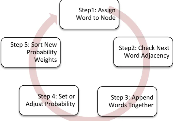
The initial for loop was the primary difference between each script. It dictated which tab delimited columns were kept and loaded into the list and which were ignored. This section was kept to a runtime of n. Sections that were useful were appended to the ex-isting section in order to keep the runtime to n. Steps are shown in Figure 3.

The next for loop checks for duplicates. It checks for empty nodes and nodes with no search entry, which were logged by some engines. We also removed any new line cha-racters and any entries that were clearly searching for a web address, although this was not robust. We decided here that interpreting users’ wills were outside the scope of this project, and while a best guess was made to strip out and sanitize our nodes, if the user wanted to search “4.jpg,” that with other unusual searches were flushed out when we calculated probabilities. Spelling errors were also outside the scope of this project, but when running the project, we found some common spelling errors to be the “most fre-quent” next node. Again, the law of numbers dictates that these difference will not be a problem, that is, frequent misspellings will yield a large enough population group that they will have a substantial data set. The final step of this loop was checking for dupli-cate entries by the same user id. We then filtered out all the empty nodes out of the list.

After this, unwanted characters were filtered out. We took all printable characters and removed the letters, numbers, space, and period, so that images would not be split into two separate nodes. We then reduced all remaining white space to a single space in an n squared operation. Then we took the final length and printed our results.

Figure 3. Steps in search query intent analysis.

Step1: Assign

Word to Node

Step2: Check Next

Word Adjacency

Step 3: Append

Words Together

Step 4: Set or

Adjust Probability

Step 5: Sort New

3. Causal Byes Net Data Structure

3.1. CBN Structure

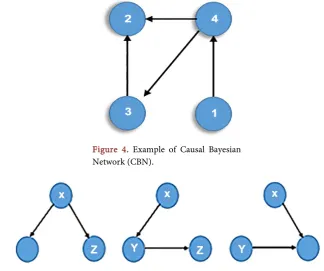
The Bayesian Network (BN) is a class of multivariate statistical models applicable to many areas in science and technology. In particular, the Bayesian Network has become popular as an analytical framework in causal studies, where the causal relations are en-coded by the structure (or topology) of the network. Causal Bayesian Network (CBN) incorporates Bayesian network in directed acyclic graph (DAG). Figure 4 shows an example of CBN with nodes and connecting edges.

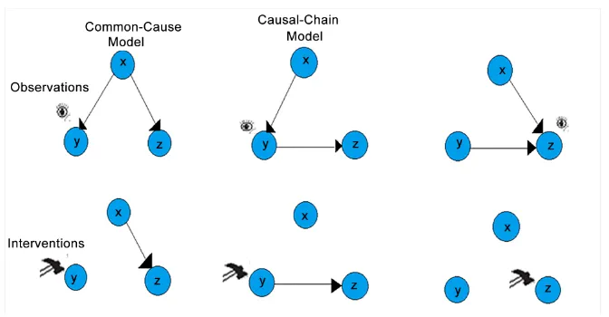
In Figure 4, Node 1 is the cause for node 4 and node 4 is the effect of node 1. Simi-larly Node 4 is the common cause for node 2 and 3. However node 3 is another cause for node. Accordingly, there are different types of CBN Models that represents com-mon cause, causal chain and comcom-mon effects that are shown in Figure 5.

3.1.1. Observations on CBN

A causal observation provides information about statistical relations among a number of events. There are three common statistical relations that represent the principle of common causes between two events “X” and “Y”: 1) X causes Y, 2) Y causes X, or both events are generated by a third event “Z” or set of events, their common cause. For example, searching for a “computer” and searching for a “computer desk” are statisti-cally related because computer causes people to go on buying a table for it. Similarly, searching for a “computer” may cause searching different computers, or printers. In searching different computers user may compare various features associated to the

Figure 4. Example of Causal Bayesian Network (CBN).

computer including the price. In these ways, a user may search ways, a computer within his/her budget or a computer with various features regardless of price. Hence, the caus-al observation of one of these events helps the model to infer that other events within the underlying causal model will exit or not.

3.1.2. Interventions on CBN

Interventions often enable us to differentiate among the different causal structures that are compatible with an observation. If we manipulate an event A and nothing happens, then A cannot be the cause of event B, but if a manipulation of event B leads to a change in A, then we know that B is a cause of A, although there might be other causes of A as well. Forcing some people to go on a diet can tell us whether the diet increases or decreases the risk of obesity. Alternatively, changing people’s weight by making them exercise would show whether body mass is causally responsible for dieting. In contrast to observations, however, interventions do not provide positive or negative diagnostic evidence about the causes of the event on which we intervened. Whereas observations of events allow us to reason diagnostically about their causes, interven-tions make the occurrence of events independent of their typical causes.

3.1.3. Counterfactual Reasoning

Counterfactual reasoning tells us what would have happened if events other than the ones we are currently observing had happened. If we are currently observing that both A and B are present, then we can ask ourselves if B would still be present if we had in-tervened on A and caused its absence. If we know that B is the cause of A, then we should infer that the absence of A makes no difference to the presence of B because ef-fects do not necessarily affect their causes. But, if our intervention had prevented B from occurring, then we should infer that A also would not occur.

3.2. Modeling Observations

inde-pendently, but once we know that X and its effect Z are present, it is less likely that Y is also present. Independence is advantageous in a probabilistic model not only because it simplifies the graph by allowing omission of a link between variables but also because it simplifies computation. Conceived as a computational entity, a Bayes net is merely a representation of a joint probability distribution—P (X, Y, Z) in Figure 5—that pro-vides a more complete model of how the world might be by specifying the probability of each possible state. Each event is represented as a variable. Causal relations have some relation to the conditional probabilities that relate events; how conditional prob-abilities and causal relations relate depends on one’s theory of the meaning of causa-tion. The factorizations of the three models at issue are:

Common cause:

(

)

(

) (

) ( )

P X Y Z =P Y X P Z X P X (1)

Causal chain:

(

)

(

) (

) ( )

Common effect:

(

)

(

) ( ) ( )

P X Y Z =P Z Y X P Y P X (3)

The equations specify the probability distribution of the events within the model in terms of the strength of the causal links and the base rates of the exogenous causes that have no parents (e.g., X in the common cause model). Implicit in the specification of the parameters of a Bayes net are rules specifying how multiple causes of a common ef-fect combine to produce the efef-fect (e.g., noisy or rule) or (in the case of continuous va-riables) functional relations between variables. A parameterized causal model allows it to make specific predictions of the probabilities of individual events or patterns of events within the causal model.

Modeling Interventions

Figure 6. Example of observations (symbolized as eyes) and interventions on (symbolized as hammers) the three basic causal models.

[29]) causal chain model with factorization of the joint distribution. With (Y =1) and do(Y = 1), observation and intervention are defined as following:

Observation of Y:

(

)

(

) (

) ( )

P X Y = Z =P Z Y= P Y= X P X (4)

Intervention on Y:

(

)

(

)

(

) ( )

P X do Y= Z P Z Y = P X (5)

Equation (4) and Equation (5) signifies that the probability of consequences of inter-ventions can be calculated if the variables of the causal model are known. Hence, it im-plies that Z occurs with the observational conditional probability, which is on the pres-ence of Y (P (Z|Y = 1), and X occurs with a probability corresponding to its base rate (P(X)). This intervention on Y is defined as the causal chain model.

CBN Models after intervention

Naturally, both of these values are significantly smaller and can be ignored for the sake of simplicity. Hence, the maximum possible entities (or event) can be represented. It is noticeable that in the natural causal effect or graph surgery fewer variables are needed to me considered in interventional probability computation. The common cause can be computed from the probability corresponding to its base rate, and the first effect is determined by the base rate of its cause and the strength of the probabilistic relation between first and second causes.

3.3. Causal Graph Data Structure

The causal graph data structure is implemented with an adjacency matrix, linked list of directions edges connections.

3.3.1. Adjacency Matrix

must be weighed to establish which is most efficient for dealing with Big Data CBN. Traditionally an adjacency matrix is the preferred method when dealing with large amounts of data so as to prevent redundant storage of values with multiple links. A problem arises in this project when the quantity of zero values is drastically greater than that of non-zero values.

Initial evaluation of word frequency using logs from all the web determined that only 9% of the 173665 unique search terms had 10 or more occurrences and thus 10 or more potential adjacencies.

Using an adjacency matrix would potentially lead to 158035 × (173665 − 10) or more than 274 billion empty values per adjacency matrix per word position. Given the in-credibly sparse nature of such an adjacency structure, an adjacency list was deemed the most appropriate option.

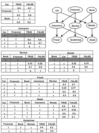
3.3.2. Truth Tables

The unique nature of search queries allowed for significant reduction in the size of the truth tables to be used in the CBN for this project. This uniqueness comes from the mutual exclusivity of search terms for each node. For example, if the word Truck is the first word used in the search term, then no other word can be true as the first word. A full-valued truth table for a given node would have a number of entries calculated by the equation in Equation (6). Where T is the number of entries in the truth table, N is the number of unique key words, and M is the word position of the current node.

NM

2

T = (6)

Reduction caused by the mutual exclusivity of the nodes in a given word position reduce this to the still large but much more manageable maximum shown in Equation (7).

(

)

T=N! N−M ! (7)

In practice both of these values are significantly smaller, these equations simply represent the maximum possible entries in a given node’s truth table.

3.3.3. Structure Layout

Due to the large volume of data, a unique data structure needed to be created. This in-cludes the establishment of a given node, the directed connection to following nodes, and the truth table needed to define the probabilities of a given state based on the ex-isting previous node states. The code for this project was written in Python with intent to eventually transfer over to LISP code. Python was used due to the robust nature of the language combined with solid readability and pre-existing functions.

Nodes were created as a Python library with the individual words as keys. These words are the initial basis for each node and are used as identifiers for both node popu-lation and forward searching for prediction methods. Due to CBN being acyclic in na-ture, a given node could not exist in more than one location so as to prevent a potential infinite loop.

method to delineate the different occurrences of the same word in different locations is needed. In order for a node to be accessed normally, the word that is keyed to the node is used as an identifier. A problem occurs in that a word could potentially exist in any word position yet must be distinct for each position else the graphs become cyclical.

Initially, a method was established to append word position to the initial key to create a unique identifier for each node. This was ultimately rejected due to the addi-tional time it would take to append this value during data mining and removal of this value for forwards searching through the nodes via string matching.

Instead, a sub-library was created within each node that would indicate the starting position based off of a non-indexed word position (starting at 1). This method sub-verted both of the problems mentioned above as the key words could maintain their string identity while still maintaining the acyclic nature of the CBN which is a directed acyclic graph (DAG). Figure 7 shows such a causal graph (DAG) generated from a sample Altavista data set.

Contained within the sub-libraries exist the word occurrence frequency (number of times that word occurs in that position), and the trimmed-down truth tables. These truth tables are calculated by dividing the number of specific occurrences of the specific path taken to reach that node by the total number of occurrences of that node in the given position.

These sub-libraries are then ranked by these probability factors during creation and modification as to reduce the total amount of time between user input and program output. Further ordering (e.g. table entries with the same values) is arbitrary and will generally be ordered chronologically by creation time.

3.4. Interpretation of Traversal

Several steps are taken in order to correctly interpret user input, search the CBN for the appropriate values, and return suggestions to the user. The initial search terms are tak-en as a single tak-entry from the user, delimited by spaces. The interpreter thtak-en counts the number of terms being used and loads the last word in the search term as the KEY. Next, both the KEY and position index are used to locate the appropriate node and po-sition to compare the entire search term to.

Once the correct truth table is located, the interpreter compares the entire string from user input until the top 5 matches have been found. These top 5 matches are re-turned as output to the user as the predictive text. The big data is proceeded through the facilities of BIG RED II from Indiana University, IN. An algorithm to convert a sample Python Code for Creation of Data Structure from CSV is shown in Figure 8 and the corresponding data structure is shown in Figure 9.

4. Results and Discussion

each search log, given the independence of the parsing of each line, this could easily be broken up to run in parallel on a supercomputer. This also allowed for all the parsed data to be combined into a single log file for breaking into data structures.

The organizing of the “mega” log into data structures took significantly less time than the parsing (only about 5 minutes for the entire log.) The primary reason these two steps were not performed in the same program was that, as individual steps, addi-tional analysis could be performed on the parsed CSV file in order to help determine the best ways to construct the data structure and to perform any secondary calculations needed to support proposed ideas.

Figure 8. Sample Python Code for creation of data structure from CSV.

The transition of the data structure to the interpreter caused some difficulty in ex-ecution. Originally the structure was sent to a Python script that would start when the interpreter was launched. This scrip file was around 400 Mb and took around four mi-nutes to load into memory. An alternative was found through Python’s Pickle functio-nality. Pickle turns a unique data structure into a binary file that Pickle can then read and load much faster when called. The result was a binary file that was only a few kb larger than the original script file, but a 50% total reduction in load time with the inter-preter.

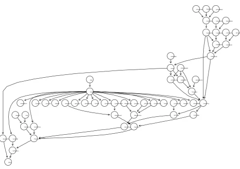
As previously mentioned, the mutual exclusivity of words in a given position reduces the storage requirements of the truth tables by a significant margin. This mutual exclu-sivity comes from the fact that two different words cannot exist in the same position. The causal nature of the CBN is also a contributing factor in the reduction of truth ta-ble sizes. Since our graph is causal, any word that never precedes a given term need not be included in our truth tables as they will never have any kind of influence on the probability of that term or word [2]. A comprehensive CBN structure is obtained while multi user search for a same item (Figure 10) and a user search difference aspect of an item (Figure 11).

Figure 10. Example CBN for multi-user search behavior towards an item (“Alltheweb” data set).

N07muVerMo SubjVertMo QGVertMotion

CombVerMo AreaMesoALS SatContMoist RaoContMoist CombMoisture AreaMoDryAir VISCloudCov IRCloudC CombClouds CldShadeOth AMInstabMt InsInMt WndHodograph OutflowFrMt MorningBound Boundaries CldShadeConv CompPlFcst CapChange LoLevMoistAd InsChange MountainFcst Date Scenario ScenRelAMCIN MorningCIN AMCINInScen CapInScen ScenRelAMIns LIfr12ZDENSd AMDewptCalPl AMInsWliScen InsSclInScen ScenRel34 LatestCIN LLIW CurPropConv ScnRelPlFcst PlainsFcst N34StarFcst R5Fcst

Figure 11. A user search behavior related to economy car in terms of “cost” “(Altavista)”.

This reduction is calculated in the worst-case-scenario in Equations (6) and (7). These are maximum models for a potential node though, and are highly unlikely to ever fully be reached. A more practical representation can be seen in Figure 7 that shows the drastic reduction in truth table size needed due to this mutual exclusivity and causation. Normally the truth tables in the third tier presented would need thirty-two separate entries to manage all possibilities. However, between the mutual exclusion and causali-ty, these tables are reduced down to between two and four values as is determined by the directed graph. It is because of all of these contributing factors that the data storage and subsequently the traversal time of such a CBN are reduced so drastically and allow for this model to be implemented in a practical way without the need for supercomputing.

The implementation of a super computer would be most strongly utilized in the farming and parsing of additional search logs. As the data is not dependant on any oth-er part during this process, it can be set up in parallel to make extensive use of any su-percomputer. The creation of the data structures could also be implemented to take advantage of such a machine, but would require more intensive modifications of the code likely involving the use of mutexs. We compared query prediction accuracy and sensitivity with some built-in Bayesian classifiers included in Weka machine learning

GoodStudent Age

Soc ioEc on

Ris k Av ers ion

Vehic leYear

This CarDam RuggedAuto

Ac c ident Mak eModel

Driv Quality

Mileage

Antiloc k Driv ingSk ill

SeniorTrain

This CarCos t

Theft CarValue

HomeBas e AntiTheft

PropCos t OtherCarCos t

OtherCar

MedCos t Cus hioning Airbag

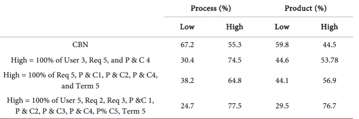
tools. Obtained results are summarized in Table 1 and Table 2.

Results in Table 1 shows the superiority of CBN based algorithms in product and process performance in terms of percentage. Table 2 shows the low and high level of sensitivity in Bayesian modeling during intentional query search.

5. Conclusions and Future Works

Many additional features could be added to this program in order to make it more robust and helpful. The most basic is the inclusion of more search logs. While this project handled about six and a half million search terms, more data will always lead to more accurate results in terms of search prediction.

A simple learning algorithm could also be implemented within the interpreter that updates the data with new search terms and reinforces existing terms as they occur. This could also potentially lead to customized terms for individual users, which would only need to create an additional mutually exclusive precondition of some forms of user ID or could, depending on the desired format, be stored locally for the user. For even further customization, a localization could also be established using a similar method so that users in a specific geographical region would be more likely to get similar results. This would be useful for things like searching for local restaurants or other geographi-cally oriented concepts.

Two significantly more robust additions could include a letter-by-letter live word prediction as the user begins to type. Google Auto-Complete implements this ability. This concept could potentially implement the same methods of prediction as the rest of the project, but we speculate that a simply ordered word frequency list would be ade-quate for this implementation. The second would be the detection and correction of

Table 1. Prediction accuracy comparison (10-fold cross-validation).

Algorithm _performance Product _performance Process Parameters Remark

CBN 77.14% 78.3%

Weka_Naive Bayes 73.65% 70.19% Default

Weka_Bayes Net 71.38 68.32% Simple estimator BAN Weka_Bayes Net 73.71% 69.55% Simple estimator TAN

Table 2. Sensitivity analysis summary.

Process (%) Product (%) Low High Low High

CBN 67.2 55.3 59.8 44.5

High = 100% of User 3, Req 5, and P & C 4 30.4 74.5 44.6 53.78 High = 100% of Req 5, P & C1, P & C2, P & C4,

and Term 5 38.2 64.8 44.1 56.9

High = 100% of User 5, Req 2, Req 3, P &C 1,

misspelled words. This would be a substantial undertaking unless pulled from some form of API, but could potentially reduce the number of nodes, and thus drastically reduce the amount of branching and storage space needed.

The final and most significant projection for this project would be following further down the Bayesian Network to obtain predictions that exceed just the next word. This would likely require a bit more search time, but not much additional coding. This would likely be implemented with a limited-depth search for ordered values. Intui-tively, the more words desired for prediction, the longer the search is going to take by a significant factor.

As discussed previously, this project could lay the groundwork for future text-based data mining for prediction usage with large data sets. Internet searching needs not be a limiting factor for the implementation of CBN with text [4]. The CBN intention recog-nition model could potentially be applied to many more concepts given the appropriate data are available. A similar network could be established using only key words that could then be used to hunt through websites, blogs, or scholarly articles to determine the intent of the entire article. This could create an automated and objective method for categorization. Such a method could potentially allow for users to input their interests to have a feed created that will direct them to, or include information they are interest-ed in. Applications of this method could also allow bloggers to more easily connect with others of similar interests.

Any implementation, such as that just mentioned, would likely need to implement selected key words so as to reduce the total number of nodes. This is due to the fact that this method would drastically reduce the need for word ordering and remove the mu-tual exclusivity that is important controlling input size of the current model.

References

[1] Pearl, J. and Varma, T. (1991) A Theory of Inferred Causation. University of California, Los Angeles.

[2] Pereira, L.M. (2011) Intention Recognition with Evolution Prospection and Causal Bayes Networks. In: Madureira, A., Ferreira, J. and Vale, Z., Eds., Computational Intelligence for Engineering Systems, Springer, Berlin, 1-33. https://doi.org/10.1007/978-94-007-0093-2_1

[3] Pereira, L.M. (2011) Elder Care via Intention Recognition and Evolution Prospection. In: Seipel, D., Hanus, M. and Wolf, A., Eds., Applications of Declarative Programming and Knowledge Management, Springer, Berlin, 170-187.

https://doi.org/10.1007/978-3-642-20589-7_11

[4] Hu, Y., Zhang, X., Ngai, E.W.T., Cai, R. and Liu, M. (2013) Software Project Risk Analysis Using Bayesian Networks with Causality Constraints. Decision Support Systems, 56, 439- 449. https://doi.org/10.1016/j.dss.2012.11.001

[5] Kvassay, M., Hluchý, L., Schneider, B. and Bracker, H. (2012) Towards Causal Analysis of Data from Human Behaviour Simulations. 4th IEEE International Symposium on Logistics and Industrial Informatics, Smolenice, 5-7 September 2012, 41-46.

https://doi.org/10.1109/lindi.2012.6319507

[7] Jiang, D., Leung, K.W.-T. and Ng, W. (2016) Query Intent Mining with Multiple Dimen-sions of Web Search Data. World Wide Web, 19, 475-497.

https://doi.org/10.1007/s11280-015-0336-2

[8] Laclavík, M., Ciglan, M., Steingold, S., Seleng, M., Dorman, A. and Dlugolinsky, S. (2015) Search Query Categorization at Scale. Proceedings of the 24th International Conference on World Wide Web, Florence, 18-22 May 2015, 1281-1286.

https://doi.org/10.1145/2740908.2741995

[9] Liu, P., Azimi, J. and Zhang, R. (2015) Contextual Query Intent Extraction for Paid Search Selection. Proceedings of the 24th International Conference on World Wide Web, Florence, 18-22 May 2015, 71-72. https://doi.org/10.1145/2740908.2742740

[10] Constantinou, A.C., Fenton, N., Marsh, W. and Radlinski, L. (2016) From Complex Ques-tionnaire and Interviewing Data to Intelligent Bayesian Network Models for Medical Deci-sion Support. Artificial Intelligence in medicine, 67, 75-93.

https://doi.org/10.1016/j.artmed.2016.01.002

[11] Chen, X., Irie, K., Banks, D., Haslinger, R., Thomas, J. and West, M. (2015) Bayesian Dy-namic Modeling and Analysis of Streaming Network Data. Technical Report, Duke Univer-sity,Durham.

[12] Acemoglu, D., Dahleh, M.A., Lobel, I. and Ozdaglar, A. (2011) Bayesian Learning in Social Networks. The Review of Economic Studies, 78, 1201-1236.

https://doi.org/10.1093/restud/rdr004

[13] Moniz Pereira, L. (2010) Anytime Intention Recognition via Incremental Bayesian Network Reconstruction.

[14] Pereira, L.M. (2013) Context-Dependent Incremental Decision Making Scrutinizing the in-tentions of Others via Bayesian Network Model Construction. Intelligent Decision Tech-nologies, 7, 293-317. https://doi.org/10.3233/IDT-130170

[15] Pereira, L.M. (2011) Intention-Based Decision Making with Evolution Prospection. In: Luis Antunes, H. and Sofia, P., Eds., Progress in Artificial Intelligence, Springer, Berlin, 254-267. [16] Armentano, M.G. and Amandi, A.A. (2009) Recognition of User Intentions for Interface

Agents with Variable Order Markov Models. In: Ricci, F., Bontcheva, K., Conlan, O. and Lawless, S., Eds., User Modeling, Adaptation, and Personalization, Springer, Berlin, 173-184.

https://doi.org/10.1007/978-3-642-02247-0_18

[17] Sadri, F. (2010) Intention Recognition with Event Calculus Graphs. IEEE/WIC/ACM In-ternational Conference on Web Intelligence and Intelligent Agent Technology (WI-IAT), 3, 386-391. https://doi.org/10.1109/wi-iat.2010.83

[18] Sadri, F. (2010) Logic-Based Approaches to Intention Recognition. In: Chong, N.-Y. and Mastrogiovanni, F., Eds., Handbook of Research on Ambient Intelligence: Trends and Perspectives, IGI Global, Hershey, 346-375.

[19] Bello, P., Cassimatis, N. and McDonald, K. (2007) Some Computational Desiderata for Re-cognizing and Reasoning about the Intentions of Others. Proceedings of the AAAI 2007 Spring Symposium on Intentions in Intelligent Systems, Stanford University, 26-28 March 2007, 1-6.

[20] Zhang, Y., Chen, W., Wang, D. and Yang, Q. (2011) User-Click Modeling for Understand-ing and PredictUnderstand-ing Search-Behavior. Proceedings of the 17th ACM SIGKDD International Conference on Knowledge Discovery and Data Mining, San Diego, 21-24 August 2011, 1388-1396.

and Knowledge Management, Maui, 29 October-2 November 2012, 2015-2019.

https://doi.org/10.1145/2396761.2398563

[22] Cui, J., Wen, F. and Tang, X. (2008) Intentsearch: Interactive On-Line Image Search Re- Ranking. Proceedings of the 16th ACM international conference on Multimedia, Vancou-ver, 26-31October 2008, 997-998. https://doi.org/10.1145/1459359.1459547

[23] Bajaj, S., Adhikari, B.M., Friston, K.J. and Dhamala, M. (2016) Bridging the Gap: Dynamic Causal Modeling and Granger Causality Analysis of Resting State Functional Magnetic Re-sonance Imaging. Brain Connectivity,Epub.

[24] Bratman, M.E. (1987) Intentions, Plans and Practical Reason. Harvard University Press, Harvard.

[25] Dasser, V., Ulbaek, I. and Premack, D. (1989) The Perception of Intention. Science, 243, 365-367. https://doi.org/10.1126/science.2911746

[26] Choi, H. and Scholl, B.J. (2006) Perceiving Causality after the Fact: Postdiction in the Temporal Dynamics of Causal Perception. Perception, 35, 385-399.

https://doi.org/10.1068/p5462

[27] Gergely, G., Nadasdy, Z., Csibra, G. and Biro, S. (1995) Taking the Intentional Stance at 12 Months of Age. Cognition, 56, 165-193. https://doi.org/10.1016/0010-0277(95)00661-H

[28] Malle, B.F., Moses, L.J. and Baldwin, D.A. (2001) Intentions and Intentionality: Founda-tions of Social Cognition. MIT Press, Boston.

[29] Hagmayer, Y., Sloman, S.A., Lagnado, D.A. and Waldmann, M.R. (2007) Causal Reasoning through Intervention. In: Gopnik, A. and Schulz, L., Eds., Causal Learning: Psychology, Philosophy, and Computation, Oxford University Press, Oxford, 86-100.

https://doi.org/10.1093/acprof:oso/9780195176803.003.0007

Appendix

Note 1: Parsing Search Data

import string

#print “What file would you like to open?” #comment this and the next line back in filename = “97_03_10.log” #raw_input(“?”)

f = open (filename, “r”) filelines = f.readlines () filedata = [len (filelines)] parsedoc = []

del f

for line in filelines:

parsedoc.append (line.strip ().split (“\t”) [1:])

#delfilelines

for i in range (len (parsedoc) −1): #this is where the magic happens if (not parsedoc [i]):

# print True continue

if (len (parsedoc[i]) = = 1): parsedoc [i] = []

continue

parsedoc [i] [1] = parsedoc [i][1].replace(“\n”, “”)

if ((parsedoc [i][1]== “”) or (“www” in parsedoc [i] [1])): #remove empty entries parsedoc [i] = []

continue

#nextline is to prevent j from reaching into the land of the lost

for j in range (i + 1, i + (20 if (20 + I < len(parsedoc)) else (len (parsedoc) −i −1))):

if (parsedoc [i] = = parsedoc [j]): parsedoc [j] = []

parsedoc = filter (None, parsedoc)

wantedchars = string.ascii_letters + “.” + string.digits unwanted = string.printable

for i in wantedchars:

unwanted = unwanted.replace (i, “”)

for i in range (len (parsedoc)): # try: parsedoc [i] [1] # except: continue for j in unwanted:

parsedoc [i] [1] = parsedoc [i] [1]. replace (j, “”) while(“ “ in parsedoc [i] [1]):

parsedoc [i] [1] = parsedoc [i] [1].replace (“ ”, “ ”)

parsedoc [i] [1] = parsedoc [i] [1].strip ()

filedata.append (len (parsedoc))

print “Originally”, printfiledata [0], print “lines.” print “Currently”, printfiledata [1], print “lines.”

for line in parsedoc: print line [0] + “,”, for word in line[1].split (“ ”): print word + “,”, print “”

Note 2: Data Structure Creation

import pickle as pl

defcreaterelations (): ourfile = “megalog”

for line in filelines:

parsedoc.append (line.strip ().split (“,”) [1:]) # for i in range(len (parsedoc [-1])):

# parsedoc [−1] [i] = “_” + parsedoc [−1] [i]

“”

Example relations-

relations = {“tree”: {1: {“branch”: 20, “stump”: 11, “”:5}{2: ...}}} “”

relations = {}

for line in parsedoc: for i in range (len (line)-1): word = line [i]

nextword = “ ”.join (line [: i + 2])

if not relations.has_key (word): relations.update ({word: {}}) posdict = relations [word] j = i + 1 if not posdict.has_key (j): posdict.update ({j: {}}) wordpos = posdict [j]

if not wordpos.has_key (nextword): wordpos.update ({nextword: 0})

wordpos.update ({nextword: wordpos [nextword] + 1})

return relations

#this section formats relations into a list that can be used with #lisp code

defformatlisp (relations): for key in relations.keys (): print “(setq”, key, “(”.strip (),

posdict = relations [key] forpos in posdict.keys (): print “(”.strip (), wordpos = posdict [pos] for word in wordpos. keys (): if not word:

else:

print “(”.strip (),word, str (wordpos [word]).strip (),“)”, print “)”,

print “))”

#formatlisp (createrelations ()) relations = createrelations ()

pl.dump (relations,open (“megafile.p”, “wb”))

Note 3: Interpreter

#from megafile import relations #from createlist import relations import pickle

fromdatetime import datetime

startTime = datetime.now ()

relations = pickle.load(open(“megafile.p”, “rb”))

defgetnext (node, numberofnext): global relations

inputlist = node. strip (). split (“ ”) #list of input words

ifrelations.has_key (inputlist [−1]):

currnode = relations [inputlist [−1]] [len (inputlist)] #dictionary from current list else:

updaterelations (inputlist) return [node, 0]

nodelist = []

fordictkey in currnode.keys ():

ourkey = “ ”.join (dictkey.split (“ ”)[: len (inputlist)]) inputkey = “ ”.join (inputlist)

if (ourkey = = inputkey):

nodelist.append ([dictkey, currnode.get (dictkey)]) #now we have [[woods, 1], [woods books.2]...]

nodelist = sorted (nodelist, key = lambda keypair: keypair [1], reverse = True)

ourrange = numberofnext if numberofnext <len (nodelist) else len (nodelist)

returnnodelist [: ourrange]

defprintnodes (nodes): pass

defupdaterelations (inputlist): pass

print "Time to load:"

printdatetime.now ()-startTime

while (1):

node = raw_input (“>>”) if node = = "/exit": exit (0)

nextnodes = getnext (str (node),5) #return a list for i in nextnodes:

print I [0]

Submit or recommend next manuscript to SCIRP and we will provide best service for you:

Accepting pre-submission inquiries through Email, Facebook, LinkedIn, Twitter, etc. A wide selection of journals (inclusive of 9 subjects, more than 200 journals)

Providing 24-hour high-quality service User-friendly online submission system Fair and swift peer-review system

Efficient typesetting and proofreading procedure

Display of the result of downloads and visits, as well as the number of cited articles Maximum dissemination of your research work