Munich Personal RePEc Archive
Testing the Lucas critique for the
Turkish money demand function
Yıldırım, Metin and Korap, Levent
Department of Economics, Faculty of Economics and Business
Administration, University of Gaziantep„ b Department of
Economics, İslahiye Faculty of Economics and Business
Administration, University of Gaziantep
2012
Online at
https://mpra.ub.uni-muenchen.de/41156/
1
Testing the Lucas Critique for the Turkish Money Demand Function
Metin Yıldırıma, Levent Korapb,*
a Department of Economics, Faculty of Economics and Business Administration, University
of Gaziantep, Gaziantep Üniversitesi İ.İB.F. İktisat Bölümü P.K. 27310 Şehitkamil, Gaziantep, Turkey
b Department of Economics, İslahiye Faculty of Economics and Business Administration,
University of Gaziantep, Hacı Ali Öztürk Mah. Mezbaha Cad. No: 3, 27800, İslahiye, Gaziantep, Turkey
Abstract. This paper aims to test the prevalence of the Lucas critique by use of an applied modelling approach. The Turkish narrow money demand is chosen for investigation purposes and an extensive statistical-based econometric application has been carried out to observe whether the model in question has been exposed to the content of such a critique. The results confirm the theory to explain the behavioral foundations of aggregate monetary economics approaches and reveal that no evidence can be found in favor of the non-rejection of the Lucas critique that leads us to infer that the modelling attempt can be considered by the researcher a feedback model which is able to encompass a whole class of expectation models.
Key Words: Money Demand; Lucas Critique; Turkish Economy; JEL Codes: C32; E41; E61;
Özet. Para talebi eşitlikleri için Lucas eleştirisinin sınanması: Türkiye ekonomisine uygulama. Bu çalışma Lucas eleştirisinin geçerliliğini uygulamalı bir modelleme yaklaşımı kullanarak sınamayı amaçlamaktadır. Türk dar para talebi araştırma amacı ile seçilmekte ve geniş kapsamlı istatistiksel-temelli ekonometrik bir uygulama sorgulanan modelin bu tür bir eleştirinin içeriğine maruz kalmış olup olmadığını gözlemlemek için gerçekleştirilmiştir. Sonuçlar kuramı derneşik parasal iktisat yaklaşımlarının davranışsal bulgularını açıklamak için doğrulamakta ve Lucas eleştirisinin reddedilememesi yönünde bir bulguyu ortaya koyamamaktadır. Bu sonuç ise bizi modelleme yaklaşımının araştırmacılar tarafından geniş kapsamlı olarak beklenti modellerini kapsayabilecek şekilde geribeslemeli bir model olarak dikkate alınabileceği çıkarsamasına götürmektedir. Anahtar Kelimeler: Para Talebi; Lucas Eleştirisi; Türkiye Ekonomisi;
JEL Sınıflaması: C32; E41; E61;
2
1. Introduction
Today’s contemporaneous economic debates witness that one of the most important issues of interest for policy makers is to provide consistency of forecasts resulted from model evaluation process with the decision making of economic agents. Related to the well-known Lucas’ critique (Lucas, 1981), since the optimal decision rules on which the structure of econometric models are based have been varied with changes in the structure of series that represent the behaviour of economic agents, the structure of econometric models used for estimation purposes will also have been altered by the systematic changes in the policy choices. That the critique holds gives rise to that comparisons of the effects of alternative policy rules using macroeconomic models will be invalid regardless of the performance of these models over the sample period or in short term forecasting.
We can easily observe that in the real world of economies, attempts to make simulations derived from empirical models coincide in many times with the application of alternative policy regimes. For applied studies, this means a structural shift in the parameters of estimated equations resulted from regime changes, and in this case, baseline regime conclusions should not be used to evaluate the effect of the control policy. That is, the Lucas critique applies (Favero, 2001). Hence, if conditional economic models have been found dependent upon specific policy actions and institutional structures of the economy though they have been estimated by using most recent or popular econometric estimation techniques, substantial changes in policies or the institutional structure may lead researchers to unwarranted estimation results and nullify the best econometric models even when the estimates seem to have desired statistical prerequisites (Stanley, 2000). In these cases subject to the regime changes and parameter instabilities, empirical studies used for estimation purposes will probably be undermined in a way leading to the invalidated policy proposals.
The concept of money demand can be considered a good candidate to examine these kind of criticisms in the economics literature. Briefly to say, money demand deals with what
motives determine the economic agents’ holding of monetary balances. Given the ex-ante
3
monetary aggregates from estimated values will likely to dominate the markets in the economy (Kontolemis, 2002). Considering these cursory appreciations for modelling purposes, we can state that conclusions derived from money demand equations are cabaple of providing crucial knowledge of how economic agents determine their behaviors of monetary holdings.
In this sense, such researches can yield estimation results informative for the constancy of money demand models which are also invariant to regime changes. Following Cheong (2003), the main difference between constancy and invariance of the applied modelling approaches is that while the former is related to the time independence of parameters, the latter would mean constancy across policy interventions both of which are among our main purposes of testing in the paper. We hope that these methodological choices in constructing and testing economic model in question will be highly useful for researchers and policy makers in search for the appropriateness of monetary stabilization policies.
This study aims to construct a conventional aggregate money demand model by employing recent developments in the time series methodologies, and for this purpose, uses data taken from the Turkish economy. Of special emphasis, in so doing, however, has been given to the stability of empirical regularities found in the data and we try to elaborately investigate whether the criticisms directed to the applied studies as summarized above can be attributed to the data realizations examined in this paper. As is briefly expressed in the following sections, there exist many papers dealing with empirical money demand models constructed upon the Turkish economy. Our paper is aimed to contribute to these studies both by re-examining the money demand function for the recent post-1998 period up to the year 2010 and by further testing the concept of non-linearity in such a function. To the best of our knowledge, there exists no paper in the Turkish economics literature applying an estimation methodology outlined in this study. We must state that in addition to the estimation of a theoretically consistent money demand model from which both conditional and marginal models are derived to test for the issues of constancy and invariance, one of the main contributions to this strand of literature is to enable the reader to observe the testing procedure of a non-linear vector error correction model also permitting smooth adjustment toward equilibrium conditions for the Turkish economy.
4
and/or financial innovation should be taken as potentially complementary explanations of a money demand instability”. Given the importance of a stable money demand relationship, many studies in recent years have been conducted on various country cases by researchers such as Sriram (1999), Kontolemis (2002), Ramachandran (2004) and Dreger et al. (2006). On the other side, Yavan (1993), Metin (1994; 1995), Üçdoğruk (1996) in this journal , Civcir (2003), Bahmani-Oskooee and Karacal (2006), Çatık (2007) in this journal and some papers by the CBRT researchers such as Mutluer and Barlas (2002), Akıncı (2003) and Altınkemer (2004) try to test the demand for money relationship for the Turkish economy.
In light of this introduction, the next section discusses some recent methodological developments to test non-linearities in time series analyses. Therefore, we extend our scope to smooth transition regression modelling to test for the existence of a non-linear equilibrium correction model for the research area in this paper. Benefited from these explanations, an application to the Turkish narrow money balances is carried out in section 3. The last section summarizes results to conclude the paper.
2. Non-linearity and Smooth Transition Regressions (STR): Conceptual Fundamentals
Since the multivariate co-integration and vector error correction methodologies as well as the related exogeneity issues are well-known in the economics literature, we omit a methodological discussion upon these subjects. But the interest readers are suggested to glance at the seminal papers of Engle et al. (1983), Engle and Granger (1987), Johansen (1988), and Johansen and Juselius (1990) or can apply to a well-mixture of these papers in Favero (2001) and Harris and Sollis (2003).
As an empirical contribution to these papers, let us briefly summarize STR framework so that we are able to test the non-linearity of error correction model derived from the co-integration relationship. Through the developments within the last two decades, we tend to follow the approaches mainly revealed by the studies of Granger and Teräsvirta (1993), and Teräsvirta (1994, 1998). The common form of STR modelling can be summarized as in Eq. 1:
´ ´ ( , ; )
t t t t t
y z z G c s (1)
where zt ( ´, ´)´w xt t is a ((m+1)x1) vector of explanatory variables with wt´ (1, yt1...,yt p )´
5
parameter vector for the linear part of the model, while is used for the non-linear parameter
vector. G(.) expresses applying to a non-decreasing and continuous transition function usually
bounded between 0 and 1, and depends on the transition variable st, the slope parameter and
the vector of location parameters c. The transition variable st can be part of zt, as one of the
explanatory variables, or of a time trend. The slope parameter >0 measures the speed of
transition between 0 and 1, and the location parameter c brings out where the transition takes
place. Observe that the model enables the researcher to begin the analysis with a linear model nested in the formulation, and permits for a further investigation to proceed with a non-linear
model specification. The most common forms of transition function of a Kth order STR model
using a logistic function with >0 and c1…ck can be written as follows:
LSTR1 Model where K=1:
1( , ; )t 1 1 st c) G c s
e
(2)
LSTR2 Model where K=2:
1 2
1 1 2 )( )
1 ( , , ; )
1 t t
t s c s c
G c c s
e
(3)
For st > ct, the transition function will approach 1 as . In the above equations, we test
non-linearity against alternative LSTR(k) models by searching for whether =0. The model is
then identified by applying to a Taylor series approximation of the transition function that was developed by Luukkonen et al. (1988). Teräsvirta (1994) derives LM-type tests of linearity
against LSTR model. A transformed auxiliary regression is used if st is an element of zt:
3
´ ´ *
0 1 j
t t j j t t t
y z
ź s (4)where (1, )´
t t
z ź . The null hypothesis of linearity would be:
0: 1 2 3 0
H (5)
The test is carried out for each of the chosen variables and the variable with the strongest
rejection against the H0 hypothesis is suggested to select as a decision rule. If non-linearity
6
0 4 3 0 3 2 3 0 2 1 2 3
: 0
: 0 0
: 0 0
H H H
(6)
An F-test is used for this purpose, and the test statistics for the null hypothesis H04, H03,H02
are estimated as F4, F3 and F2, respectively. In line with Teräsvirta and Eliasson (2001), our
decision rule is based on the inference that if the p-value of the test of H03 is rejected more
strongly than H02 and H04, we tend to decide the use of an LSTR(2) model, otherwise an
LSTR(1) model will be chosen. In case the test sequence cannot yield unambigious results, the researcher can scrutinize the relevant information criteria or the residual sum of squares.
Note that in the LSTR formulation, the parameters will change monotonically with the
transition function with asymmetric adjustment toward equilibrium, and as , the model
becomes a two-regime switching model. Whereas, in exponential STR (ESTR) models, the adjustment would be symmetric around long run equilibrium as is in Eq. 7:
2
( )
( , ; ) 1 st c
t
G c s e , >0 (7)
3. Empirical Findings
3.1. Preliminary Data Issues: Definitions and Time Series Characteristics
Following the theoretical bases summarized in the former sections, a money demand model using the Turkish data is constructed. For this purpose, the sample period with quarterly observations lies between 1998Q1 and 2010Q4. The motivation of the starting point is the use of 1998: 100 based new income series to extract the price data derived from gross domestic
product (GDP) deflator (p). The monetary variable (m) is the narrow money balances, which
7
rate representing the increase of prices of intangible assets. Given these choices, the scale
income variable (y) for the maximum amount of money balances to be held in hand is the real
GDP data at constant 1998 prices. The interest rate variable (i) is an average interest rate on
securities in Treasury actions to represent returns on financial assets. For the effect of the course of equity prices on money demand equation, the Istanbul Stock Exchange (ISE)
National-100 index (eq) is considered. Further, putting a variable representing currency
substitution or dollarization phenomenon in a money demand functional form may be important especially in an inflationary environment. Such a variable will reflect the extent to which policy authority loses domestic monetary control when the demand for foreign exchange increases in the economy. For this purpose, the Turkish lira / US dollar exchange
rate (e) is included into the analysis.
We must state that within the estimation process, we have observed that adding a price variable converted into inflationary developments as an alternative cost besides the interest rate has been resulted in a contradictory inverse sign due possibly to a multicollinearity problem between these aggregates, but putting one of them as a single variable has given us a theory-consistent functional relationship. Therefore, we decided to proceed with interest rate and dropped the inflation variable from the money demand equation. Finally, the own return of money balances is assumed to be zero for the narrow money demand. All the data except the interest rates are used in their natural logarithms and indicate seasonally unadjusted
values. For the variables m, y, eq and e, the source is the electronic data delivery system of the
Central Bank of the Republic of Turkey (CBRT), while data for interest rate variable i are
compiled from the electronic data delivery system of the Turkish Republic Prime Ministry State Planning Organization. The underlying model can be expressed as follows:
1 2 3 4
(m p)t ct yt it e qt et t (8)
where t is a priori asumed to be a white noise error term.
8
Using non-stationary variables in estimation process will likely to produce the
so-called spurious regression problems in conventional ordinary least squares (OLS) estimation
[image:9.595.71.521.352.567.2]techniques that strongly lead the variables to diverging from long run means with biased standard errors and result in unreliable correlations and unbounded variance processes. Also, the existence of structural breaks in time series would make it difficult to discern definitive properties in a variable form. Therefore, we first conduct some unit root tests suggested by Dickey and Fuller (1981) assuming no structural break, Zivot and Andrews (1992) assuming one endogenous break and Lumsdaine and Papell (1997) that allow for two endogenous breaks. To save space, we have omitted methodological discussion upon these tests. In Table 1, Both the ADF, ZA and LP tests, for which the latter two tests can be referred to as C and CC models, are not able to reject the unit root null hypothesis in the level form variables:
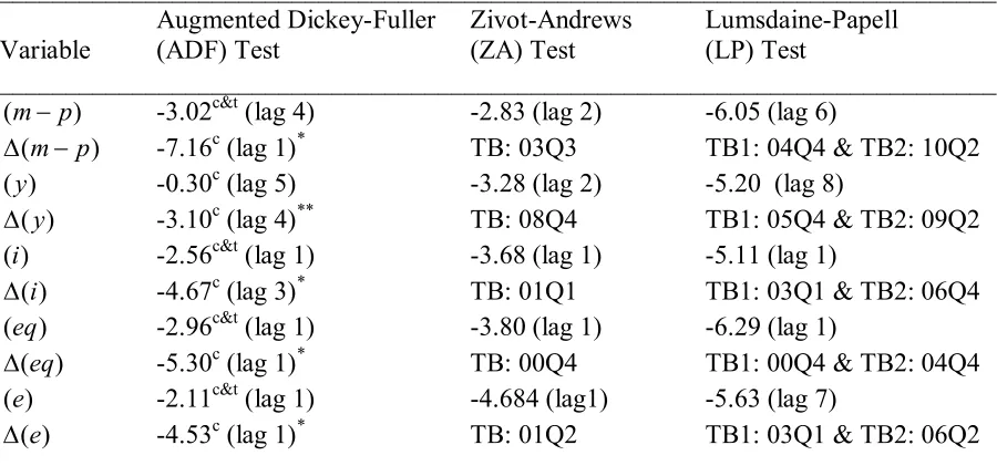
Table 1. Univariate unit root tests
___________________________________________________________________________
Augmented Dickey-Fuller Zivot-Andrews Lumsdaine-Papell
Variable (ADF) Test (ZA) Test (LP) Test
___________________________________________________________________________
(m p ) -3.02c&t (lag 4) -2.83 (lag 2) -6.05 (lag 6)
(m p)
-7.16c (lag 1)* TB: 03Q3 TB1: 04Q4 & TB2: 10Q2
( )y -0.30c (lag 5) -3.28 (lag 2) -5.20 (lag 8)
( )y
-3.10c (lag 4)** TB: 08Q4 TB1: 05Q4 & TB2: 09Q2
( )i -2.56c&t (lag 1) -3.68 (lag 1) -5.11 (lag 1)
( )i
-4.67c (lag 3)* TB: 01Q1 TB1: 03Q1 & TB2: 06Q4
( )eq -2.96c&t (lag 1) -3.80 (lag 1) -6.29 (lag 1)
( )eq
-5.30c (lag 1)* TB: 00Q4 TB1: 00Q4 & TB2: 04Q4
( )e -2.11c&t (lag 1) -4.684 (lag1) -5.63 (lag 7)
( )e
-4.53c (lag 1)* TB: 01Q2 TB1: 03Q1 & TB2: 06Q2
___________________________________________________________________________
Notes: In the ADF test * and ** indicate the rejection of the null hypothesis for the 1% and 5% levels,
respectively. c and c,t represent the allowance for only constant and constant&trend terms as deterministic
components, respectively. is the difference operator and yt yt - yt-1y; k is the number of lags determined
for each possible breakpoint by minimizing the Schwarz Bayesian information criteria and t is assumed to be
i.i.d. error term. The critical vales for the ZA test are -5.57 (1%) and -5.08 (5%). The critical valus for the LP test equal -7.19 (1%) and -6.75 (5%), which are taken from the paper of Ben-David et al. (2003).
3.2. Rank Analyses and Evidence for VAR-Based Multivariate Co-integration
9
in the model estimation process, a set of centered seasonal dummies which sum to zero over a
year are used. Further, an impulse dummy variable (dummy01) which takes on values of unity
from 2001Q1 to 2001Q4 is attributed to the macroeconomic crisis conditions experienced by the Turkish economy. These dummies in the model enter the system in an unrestricted way, because, we do not expect them to have long-run effects endogenous to the specification of the variable vector. An intercept and trend factor are restricted into the long-run variable space as exogenous variable for the deterministic part of the model, but we do not assume a quadratic deterministic trend lying in both the co-integrating model and the dynamic VEC model since allowing for linear trends in the short-run VEC model possibly leads the researcher to be obliged to rationalize why an implausible ever-increasing or decreasing rate of change dominates the data in an economic sense. We will see below that such a choice of restricting trend factor into the system yields significant estimation results so that attemts to drop this deterministic term from the model will be a lack of researcher to catch the true data generation process derived from our applied modelling. The long-run co-integrating relationships between the variables are estimated by using two likelihood test statistics known
as maximum eigenvalue for the null hypothesis of r versus the alternative of r+1
co-integrating relationships and trace for the null hypothesis of r against the alternative of n
co-integrating relations, for r = 0,1, ... , n-1 where n is the number of endogenous variables.
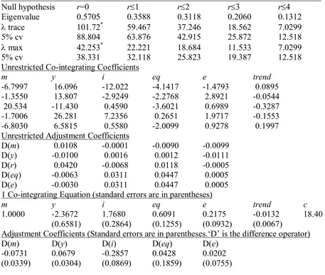
Based on the critical values taken from Osterwald and Lenum (1992) and on newer p
-values from the study of MacKinnon et al. (1999), in Table 2 in Appendix, we first try to determine the rank order of the model for the existence of possible statistically significant co-integrating vectors. In the upper part of the table can easily be observed that against the null hypothesis of no co-integration in the multivariate model we are unable to reject that there exists a unique co-integrating relationship lying in the long-run variable space estimated by both maximum likelihood statistics, thus, some combinations of the I(1) variables of our interest tend to yield a stationary relationship. The unrestricted co-integrating coefficients
indicate that the first row with the largest eigenvalue statistic seems to satisfy the a priori
theory-based expectations for a conventional money demand model, since all the variables carry quitely plausible coefficients to which economic interpretations in Eq. (8) can be imposed and are found with statistically significant normalized signs with regard to the real money balances:
10
We estimate that the real income elasticity of money balances under the money market equilibrium conditions is 2.37, which is obviously larger than a unitary coefficient. Following Sarno (1999), on this point, we can suppose that the disequilibria between real income and real money balances will affect the current demand conditions through the inverse monetary
velocity measure (m-p-y). If real income elasticity equals unity in a long-term stationary
relationship, which can also be tested by employing homogeneity restrictions, acceptance of this assumption will give support to the quantity theoretical approaches that assume a strong proportional relationship between real income and real balances to provide a stationary income velocity of monetary aggregates. If real income elasticity takes values between one-half and unity, such a finding will be consistent with the economies of scale argument put forward in the context of the inventory-theoretic transactions models. On this issue, see e.g. Ozmen (1998) estimating a currency seigniorage model for the Turkish economy. On the other hand, if real income elasticity is significantly above unity as is found in our study, which will indicate an increasing ongoing monetization process in the economy, demand for real money balances can be considered like a demand for luxury goods, which will be resulted in declining monetary velocity. Such a finding should not be surprising for the Turkish economy, since inside the sample period of 1998-2010 an obvious downward tendency in domestic inflation dominates the economy. Let us note here that in a consistent way to the above findings, the unit real income homogeneity restriction cannot be accepted for the 5%
significance level using the estimation results of 2(1)=3.0185 against the table-value
2(1)=3.8415.
Besides the real income scale variable, the most significant alternative cost variable is found as the semi-elasticity of the Treasury interest rate with a normalized coefficient -1.7680 followed by the coefficients of equity price and exchange rate variables which take the estimation values -0.6091 and -0.2175, respectively. These results confirm the empirical success of the theory to explain the behavioral foundations of aggregate data-supported monetary economics approaches. We find a significant positive trend which implies that agents’ demand for real money balances has an increasing tendency in the sample period.
11
respectively, are statistically significant. For the adjustment coefficients of equity prices and exchange rate, we are unable to reject the null hypothesis of being weakly exogenous, thus, these variables cannot be warranted in a dynamic VEC equation to include the relevant error correction term constructed upon them. Such a case means explicitly that the main factors leading to the weakly exogenous variables are determined out of the money demand variable
space. Note also that the joint weak exogeneity restriction for the variables m, y and i cannot
be accepted by using a 2(3)=19.373 (prob. 0.0002) statistic, but the joint weak exogeneity of
the variables eq and e are valid by using a 2(2)=0.1567 (prob. 0.9247) statistic.
3.3. Sensitivity to Endogenous Break in the Co-integration Space: Gregory-Hansen Evidence
In the former section, we explore that it is possible to construct a theory consistent co-integrating relationship of the same order integrated variables. However, in a similar way to the unit root analysis, there may be a question of structural shifts in the estimated relationship. For this purpose, we follow the methodology proposed by Gregory and Hansen (henceforth GH) (1996a, 1996b) which enable the researcher to test an endogenously determined break point chosen by the data structure of the model. GH test is an extension of the Engle and Granger (1987) co-integration methodology and proposes a residual based approach to statistically examine the presence of one unknown shift for the null hypothesis of no co-integration against the alternative of co-co-integration with a break. We will consider three alternative models which are Model C with a level shift, Models C/T with a level shift with trend, and Model C/S with a regime shift that allows the slope vector to shift:
1 2
1 2
1 2 1 2
M o d el C : L evel sh ift = + + +
M o d el C /T : L evel sh ift w ith tren d = + + + M o d el C /S : R eg im e sh ift = + + +
t t t t
t t t t
t t t t t t
y X
y t X
y X X
t = 1, …, n (10)
where:
0 if 1 if
t
t n t n
(11)
The unknown parameter (0,1) represents the relative timing of the change point, and equals
12
shift, 2 the change in the intercept at the time of the shift, the coefficient of the time trend,
1 the co-integrating slope coefficient before the regime shift and 2 the change in the slope
coefficient. Following GH (1996a), the test statistics in Eq. 12 is computed for each break
point (T) in the interval ([0.15n], [0.85n]) recursively, and the smallest value is chosen:
* *
*
in f ( ) i n f ( )
in f ( ) T
t T t
T
Z Z
Z Z
A D F A D F
(12)
Above, Z* and *
t
Z give the minimum values of the relevant Phillips test statistics, and ADF*
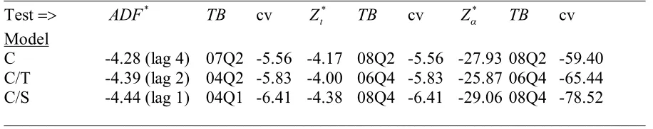
[image:13.595.68.526.343.434.2]is the minimum value of the ADF test. The results are given in Table 3:
Table 3. GH Test for Structural Shift in the Co-integrating Relationship
___________________________________________________________________________
Test ADF* TB cv *
t
Z TB cv Z* TB cv
Model
C -4.28 (lag 4) 07Q2 -5.56 -4.17 08Q2 -5.56 -27.93 08Q2 -59.40
C/T -4.39 (lag 2) 04Q2 -5.83 -4.00 06Q4 -5.83 -25.87 06Q4 -65.44
C/S -4.44 (lag 1) 04Q1 -6.41 -4.38 08Q4 -6.41 -29.06 08Q4 -78.52
___________________________________________________________________________
Notes:
1 For the autoregressive lag structure of the ADF model, the Bayesian information criterion (BIC) is used. 2 5% critical values (cv) assume four regressor case (m = 4), and TB indicates the estimated break date.
The results reveal that we cannot reject the null hypothesis of no co-integration relationship at the 5% significance level, and there exists no endogenous structural break subject to the long-run money demand variable space. Had there not been found evidence of stability in the co-integration analysis, we would have been obliged to estimate the long-run money demand equation for each sub-period considering pre- and post-break sample dates inclusive of related dummy variables. Fortunately, on no account do we have to interest in such an instability issue. We will examine the single equation conditional error correction model.
3.4. The General-to-Specific Single Equation Conditional Error Correction Modelling
13
to the one-period lagged knowledge of the co-integrating relationship, as the error correction term, and centered seasonal dummies:
1 1 1 1 1 1 1 2 1 3 1 4
5 6 7 8 9
1 1
( ) [( ) )] ( ) ( ) ( )
( ) ( ) _ 2 _ 3 _ 4
t t t t t t t i t i i t i i t i
t i t i t
i i
D m p c m p y i eq e D m p D y D i
D eq D e D Q D Q D Q
(13)where the long term co-integrating relationship is indicated in [ ], and ‘D’ represents the first
difference operator. For the dynamic lag structure, we follow the long-run model with the use
of lag order 1. t is again assumed to be a white noise disturbing term. To eliminate the
over-parametrization, we present the reduced form model below for which statistically insignificant
variables are sequentially dropped by applying to redundant variables F-test, and
parsimonious error correction model only with the econometrically meaningful variable results are obtained:
1 1 1Redundant Variables (4,38)-statistic= 0.2006 Prob. 0.9364 White Heteroskedasticity-Consistent SEs and Covariance in ()
0.0230 0.0791 t 0.1010 ( )t 0.0741 ( )t 0.0963 _ 2 0.1446 _ 3 0.07 t
F
D m p EC D i D eq D Q D Q 15 _ 4
(0.0052) (0.0341) (0.0439) (0.0272) (0.0128) (0.0216) (0.0155) L statistics [0.0936] [0.0569] [0.416i
D Q
2
3] [0.1882]
Adj.R 0.6339, Std. Error of Regression = 0.0341, SSR=0.0489, stat.=14.8529 (Prob. 0.00), D-W stat.=1.9859, B-G AR(1) stat.=0.0355 (Prob. 0.8514), B-G AR(4) stat.=
F
F F
0.0879 (Prob. 0.9857), J-B=0.1649 (Prob. 0.9208),
White stat.=1.3413 (Prob. 0.2338), ARCH(1) stat.=2.5566 (Prob. 0.1167), ARCH(4) stat.=1.3127 (Prob. 0.2818), Ramsey RESET stat.=1.9254 (Prob. 0.
F F F
F
1728)
Above, Li is the Hansen (1992) individual stability test statistics, while Lc is the joint
stability test statistic of the coefficients and error variance. Under the null hypothesis of
parameter stability, 5% asymptotic critical value for the Li test with 1 degree of freedom
(d.o.f.) is 0.47, and 5% asymptotic critical value for the joint test with m+1=8 d.o.f. is 2.11 where m represents the regression parameters. Consider that the dummies are dropped from the equation when the breakpoint tests are carried out.
14
15% trimming is chosen where the first and last 7.5% of the observations are excluded for estimation purposes. The results vare given in Table 4 below:
Table 4. Quandt-Andrews Breakpoint Tests
__________________________________________________________________________________
0:No breakpoints within trimmed data
Equation Sample: 1998Q4 2010Q4 Test Sample: 2000Q1 2008Q1 Number of breaks compared: 33
Max. LR stat.(2003Q2)=2.6631 (Prob. 0.9999), Max. Wald stat.(2005Q1)=3.522
H
F F 9 (Prob. 0.9943),
Exp LR stat.=0.6240 (Prob.0.9999), Exp Wald stat.=1.0347 (Prob.0.9516), Ave LR stat.=1.1172 (Prob. 0.9999), Ave Wald stat.=1.7948 (Prob. 0.9468)
Hansen's Instability Tests Vari
F F
F F
ance: 0.2920 Joint Statistic : 1.4843Lc
___________________________________________________________________________
In a supporting way the co-integration results in Table 2, we find that nearly 7.9% of the adjustment in money demand disequilibrium conditions to long-run static equilibrium is realized within one period. We obtain significant coefficient estimates for one-period lagged values of the differenced interest rate and equity price variables. The model is highly well-behaved as for the diagnostics and whitens satisfactorily the residual structure of the parsimonious error correction equation. No unknown breakpoint can be seen in the equation.
Further, Hansen (1992) coefficient stability L test results given above reveal both the stability
of the individual coefficients and the joint stability of the coefficients and the estimated variance.
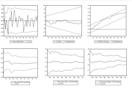
15
[image:16.595.77.523.160.467.2]results nor recursive coefficient estimates support any evidence in favor of parameter or variance instability:
Figure 1. Recursive Estimates for the Linear Conditional Error Correction Model
___________________________________________________________________________ -.100 -.075 -.050 -.025 .000 .025 .050 .075 .100
01 02 03 04 05 06 07 08 09 10 Recursive Residuals ± 2 S.E.
-20 -15 -10 -5 0 5 10 15 20
01 02 03 04 05 06 07 08 09 10 CUSUM 5% Significance
-0.4 -0.2 0.0 0.2 0.4 0.6 0.8 1.0 1.2 1.4
01 02 03 04 05 06 07 08 09 10 CUSUM of Squares 5% Significance
-.20 -.16 -.12 -.08 -.04 .00 .04
02 03 04 05 06 07 08 09 10 Recursive EC(t-1) Estimates ± 2 S.E.
-.4 -.3 -.2 -.1 .0 .1 .2
02 03 04 05 06 07 08 09 10 Recursive Dr(t-1) Estimates ± 2 S.E.
-.2 -.1 .0 .1 .2 .3
02 03 04 05 06 07 08 09 10 Recursive Deq(t-1) Estimates ± 2 S.E.
___________________________________________________________________________
3.5. Testing for Super Exogeneity and Marginal Modelling
In the system co-integration analysis carried out in the former sections, we find that there
exist two weakly exogenous variables, i.e., equity prices (eq) and exchange rate (e), lying in
the long-run variable space. Under the assumption of a single co-integrating vector derived from a constrained maximum likelihood problem, in Table 2, we are unable to reject the joint hypothesis that the two unrestricted adjustment or loading coefficients for these variables are
zero, which is inferred from a 2=0.1567 (prob. 0.9247) statistic. Further, no evidence against
16
invariant to the class of interventions occuring during the sample period or that they can be reliable estimators against instabilities resulted from regime changes. This means that models based on backward looking behaviors would not be resulted in constant conditional models if they have been exposed to violent variations in the parameter structures. Considering these prerequisities for a complete modelling, Hendry and Ericsson (1991b) using a general-to-specific approach try to obtain constant error correction framework against the instability of money demand models and also apply to the super exogeneity tests to examine the invariance property in the sense of the Lucas critique.
In order to conduct a policy analysis, as Favero and Hendry (1992) point out, only through the researcher satisfies the property that the parameters of the model are invariant to changes in the distribution of the weakly exogenous conditioning variables can we arrive at the inference that these variables have also been of a super exogeneity form. This requires constructing marginal models using these variables on which the money demand model has been conditioned, then, the super exogeneity assumption can only be rejected if the constructed variables derived from the marginal models have no statistical significance on the conditional model. Provided that the super exogeneity property can be obtained the researcher will gain a more robust degree of autonomy in policy conducting analyses by changing the processes driving these policy variables.
17
Following the explanations in the studies of Hendry (1988) and Engle and Hendry (1993), in this section, the super exogeneity tests are tried to be applied. To the best of my knowledge, Metin (1995) chosen to be followed in our estimation process is an extensive study that deals with the empirical findings of super exogeneity and the Lucas critique for the Turkish economy. To examine whether non-constancies in the marginal models for conditioning variables are able to affect the conditional model in a significant way, we first construct univariate fifth order autoregressive marginal models for the weakly exogenous
contemporaneous variables eqt and et. Then, we calculate the recursive residuals followed by
some Chow instability tests and assign dummies for the periods that reflect structural breaks and instabilities included into the data. The calculated dummies and the residuals extracted from the marginal models are added into the conditional error correction model so as to test invariance and super-exogeneity, respectively. The parsimonious marginal models are given below (White HCSEs in parentheses),
1 5
2
1:Marginal equation
Redundant Variables (3,40)-statistic= 0.2744 Prob. 0.8435
0.0575 0.2693 0.3298
(0.0245) (0.1208) (0.1608)
Adj.R 0.2038, Std.
t
t t t
Model D eq F
D eq D eq D eq
Error of Regression = 0.1616, SSR=1.1228, stat.=6.7579 (Prob. 0.00), D-W stat.=1.9425,
B-G AR(1) stat.=0.1659 (Prob. 0.6860), B-G AR(4) stat.=0.5352 (Prob. 0.7107), J-B=0.0124 (Prob. 0.9938),
Whi
F
F F
te stat.=3.0606 (Prob. 0.0045), ARCH(1) stat.=0.1738 (Prob. 0.6788), ARCH(4) stat.=0.9293 (Prob. 0.4576),
Ramsey RESET stat.=6.6164 (Prob. 0.0140)
F F F
F
1 5
2
2 : Marginal equation
Redundant Variables (3, 40)-statistic= 0.0781 Prob. 0.9715 0.0064 0.3340 0.2714
(0.0136) (0.1118) (0.0989)
Adj.R 0.1821, Std. Error of t
t t t
Model D e F
D e D e D e
Regression = 0.0872, SSR=0.3270, stat.=6.0105 (Prob. 0.00), D-W stat.=2.0084, B-G AR(1) stat.=0.0054 (Prob. 0.9417), B-G AR(4) stat.=0.1632 (Prob. 0.9557), J-B=60.2750 (Prob. 0.0000), White st
F
F F
F
at.=0.6234 (Prob. 0.6827), ARCH(1) stat.=0.2475 (Prob. 0.6214), ARCH(4) stat.=0.3190 (Prob. 0.8634), Ramsey RESET stat.=1.4047 (Prob. 0.2426)
F F
F
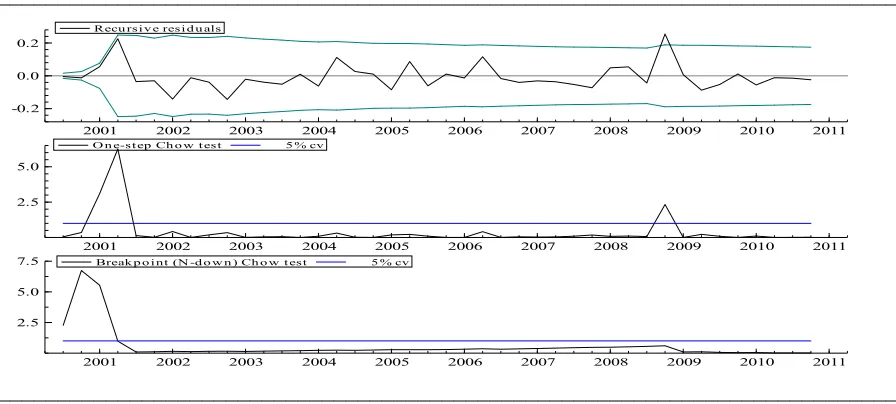
The one-step residuals and one-step Chow test results using recursive least squares estimators are figured out to determine possible instabilities. In Figure 2, the recursive
residuals lie outside the 2 S.E. bands for the 2008Q4 period with a coefficient -0.3716 (S.E.
0.1720), recursive one-step Chow tests yield significant F-stat. (1,4) = 66.640 (prob. 0.0012)
18
recursive breakpoint (N-down) tests result in respective F-stat. (41,2) = 24.535 (prob. 0.0399)
for the 2000Q4 period and F-stat. (39,4) = 7.3621 (prob. 0.0319) for the 2001Q2 period. For
the marginalD e
model, the recursive residuals again lie outside the 2 S.E. bands for the2008Q4 period with a coefficient 0.2548 (S.E. 0.0943), recursive one-step Chow tests yield
significant F-stat. (1,3) =31.377 (prob. 0.0112) for the 2001Q1 period, F-stat. (1,4) = 48.231
(prob. 0.0023) for the 2001Q2 period and F-stat. (1,34) = 9.6289 (prob. 0.0038) for the
2008Q4 period, and finally recursive breakpoint (N-down) test result in respective F-stat.
(42,1) = 570.84 (prob. 0.0332) for the 2000Q3 period, F-stat. (41,2) = 131.28 (prob. 0.0076)
[image:19.595.74.522.329.521.2]for the 2000Q4 period and F-stat. 47.637 (prob. 0.0042) for the 2001Q1 period:
Figure 1. Recursive Tests for D eq
equation___________________________________________________________________________
2001 2002 2003 2004 2005 2006 2007 2008 2009 2010 2011
-0.5 0.0
0.5 Recu rsi v e resi d u als
2001 2002 2003 2004 2005 2006 2007 2008 2009 2010 2011
2.5 5.0
7.5 O n e-step Ch o w t est 5% cv
2001 2002 2003 2004 2005 2006 2007 2008 2009 2010 2011
0.5 1.0
Break p o in t (N -d o w n ) Ch ow t es t 5 % cv
___________________________________________________________________________
Figure 2. Recursive Tests for D e
equation___________________________________________________________________________
2001 2002 2003 2004 2005 2006 2007 2008 2009 2010 2011
-0.2 0.0 0.2
Recu rsi v e resi d u als
2001 2002 2003 2004 2005 2006 2007 2008 2009 2010 2011
2.5 5.0
O n e-st ep Ch o w t est 5 % cv
2001 2002 2003 2004 2005 2006 2007 2008 2009 2010 2011
2.5 5.0
7.5 Break p o i nt (N -d o w n ) Ch o w t est 5 % cv
[image:19.595.72.520.568.770.2]19
Then, we have re-estimated the marginal models by including zero / one shift dummies to account for instabilities:
1 5
Redundant Variables (4,38)-statistic= 0.2500 Prob. 0.9079
0.0675 0.2397 0.3229 0.3947 2
(0.0231) (0.1184) (0.1592) (0.0274)
t t t
F
D eq D eq D eq mardummy
1 5
Redundant Variables (3,38)-statistic= 0.2836 Prob. 0.8369
0.0081 0.3326 0.2329 0.1172 1 0.2730 2
(0.0122) (0.1120) (0.1123) (0.0392)
t t t
F
D e D e D e mardummy mardummy
(0.0733)
where mardummy1 takes unity for the 2000Q3, 2000Q4, 2001Q1 and 2001Q2 periods and is
zero otherwise, and mardummy2 takes unity for the 2008Q4 period and is zero otherwise. As
can be clearly noticed, the both dummies capture the upward tendency in exchange rate for the instability periods. Also, the negative impact on the stock exchange is highly evident in the 2008Q4 period. Having estimated these generated regressors, we follow Hurn and Muscatelli (1992) and carry out the super exogeneity tests by additionally including residuals
extracted from the marginal models (reseq and rese, respectively) plus the dummies that
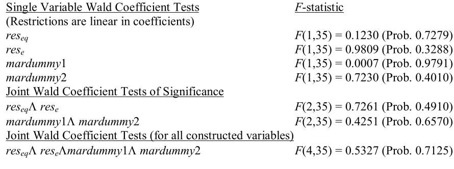
[image:20.595.65.510.483.649.2]account for the concept of invariance into the conditional error correction model in Table 5:
Table 5. Superexogeneity tests for the generated regressors in the conditional EC model ___________________________________________________________________________
Single Variable Wald Coefficient Tests F-statistic
(Restrictions are linear in coefficients)
reseq F(1,35) = 0.1230 (Prob. 0.7279)
rese F(1,35) = 0.9809 (Prob. 0.3288)
mardummy1 F(1,35) = 0.0007 (Prob. 0.9791)
mardummy2 F(1,35) = 0.7230 (Prob. 0.4010)
Joint Wald Coefficient Tests of Significance
reseq rese F(2,35) = 0.7261 (Prob. 0.4910)
mardummy1 mardummy2 F(2,35) = 0.4251 (Prob. 0.6570)
Joint Wald Coefficient Tests (for all constructed variables)
reseq resemardummy1 mardummy2 F(4,35) = 0.5327 (Prob. 0.7125)
___________________________________________________________________________
20
for marginal model instability points. These results mean that the conditional error correction model has not been exposed to parameter non-constancies that yield evidence for the Lucas critique and that it can be considered a feedback model which is able to encompass a whole class of expectation models.
3.6. Testing for Non-Linearity in the EC Equation
As a final stage in our applied paper of the Turkish narrow money demand, we will try to test the linearity of the baseline parsimonious error correction equation against the relevant non-linear STR version. In the original equation above, we find that the RESET test cannot reject the null hypothesis of no mis-specification in the parsimonious linear EC model. If not so, the model would be able to require a higher order polynomial functional form inclusive of, e.g., quadratic and/or cubic terms. As Granger and Teräsvirta (1993) emphasize, this test can be considered an LM test of linearity against a very special modelling approach of the STR type. Thus, we further aim to conduct some tests of the logistic STR model to control the data consistency, so we can infer in a more robust way whether the estimation procedure can be improved by additionally modelling non-linearity.
For this purpose, we first examine the null hypothesis of linearity for the parsimonious
conditional error correction model and test that H0:12 3 0against the alternative
non-linearity hypotheses. Note that the constant term and centered seasonal dummies are allowed to enter the linear part of the model as is in the original error correction
representation. Each of the variables ECt1,D i
t1, and D eq
t1 are used as transitionvariables in turn. The results are reported in Table 6 below:
Table 6. p-values of the Linearity Tests of the Conditional EC Equation
___________________________________________________________________________
1 1 1
0
Testing Linearity against STR
Variables in AR part: constant ( ) ( ) _ 2 _ 3 _ 4 Sample range: [1998Q2 2010 Q4], =51
values of -tests
Transition Variable H
t t t
EC D i D eq D Q D Q D Q
T
p F
04 03 02
1
H H H Suggested Model 2.5198e-01 5.6440e-01 1.1946e-01 3.1053e-01 Linear
t EC D
1 1
( ) 3.6151e-01 6.3549e-01 4.7655e-01 9.5739e-02 Linear ( ) 8.7555e-01 6.6726e-01 8.4998e-01 5
t
t i D eq
.8017e-01 Linear
21
In the table, we do not succeed in rejecting the H0 hypothesis since the relevant p
-values for all the possible transition variables cannot reach the acceptable significance levels to keep on an analysis of non-linearity in our applied modelling approach. Thus, we choose to retain the specification of the linear error correction model of the money demand as the warranted time series estimation process against the alternative STR modeling attempts. However, it must be stressed out that due to the preliminary investigation of the time series in the former sections, we do not include inflation data realizations into the estimation process, but various other model specifications different than the application in this study can make a model formulation inclusive of the inflation rate possible as the alternative cost variable of money demand.
4. Conclusions, Policy Discussion and Suggestions for Future Researches
One of the most important issues of interest for today’s macroeconomic debates is to reveal the stability of functional relationships upon which economic theories are constructed and tested by using popular estimation techniques. If constancy of the models cannot be provided,
the ex-ante model evaluation process will not possibly reflect the true data generation process
to test the motives used for decision making of economic agents and to infer what policies are appropriate for stabilization purposes under the whole periods examined. In this paper, we have tried to examine such a policy issue mostly highlighted by the Lucas critique in the economics literature for the narrowly defined money demand relationship in the Turkish economy. We have thus aimed at testing whether the money demand relationship has been exposed to the structural breaks and parameter instabilities that give rise to regime changes.
22
as to improve our empirical model. Of all the variables, the weak exogeneity property in a system co-integration relationship cannot be rejected for the equity prices and exchange rate, thus, we have applied marginal modelling procedure constructed on these variables to test whether they are really of the conditioning form in the VEC estimation. The results reveal that no evidence can be found in favor of the rejection of the super exogeneity property of the equity prices and exchange rate variables which means that the conditional EC model has not been exposed to in-sample parameter non-constancies that yield evidence for the Lucas critique and that it can be considered a feedback model which is able to encompass a whole class of expectation models. The linearity in the conditional error correction model cannot be rejected as the warranted time series estimation against the alternative non-linear models.
If theory-backed empirical models are able to be estimated by the researchers, these findings will give a change to the policy makers in order to have a foresight for the possible
outcomes of ex-ante designed policies. Such an inference has been of a special importance
especially in monetary theory analyses. In this line of thought, since we are succeed in estimating a stable narrow money demand model which is not fortunately subject to the contemporaneous Lucas critique mainly directed to the econometric applications of the researchers, we can state that our findings tend to increase the autonomy of policy makers at first to control the course of the monetary aggregates and then to use them for various stabilization purposes, e.g. in fighting inflation. But, the readers do consider the issue that our findings in the paper reflect a general tendency of the data restricted for our sample period. However, and of course if possible, the extension of the time series for the earlier and later periods can yield results violating super exogeneity and invariance property of the estimated model due to possible policy regime changes. We think that this is the critical issue to understand the main theme of this paper and to derive various policy outcomes from such empirical studies.
23
In this empirical economics paper, a set of econometric procedures available in the software programs EViews 6.0., STATA 9.0., Gauss 10.0., PcGive 10.40. and JMulTi 4.24 are tried to be used for econometric modeling purposes.
The authors would like to thank anonymous referee(s) for their leading criticism and suggestions in constructing this paper. The usual disclaimer applies.
[image:24.595.69.526.283.670.2]APPENDIX
Table 2. Multivariate co-integration analysis (restricted linear deterministic trend)
___________________________________________________________________________
Null hypothesis r=0 r1 r2 r3 r4
Eigenvalue 0.5705 0.3588 0.3118 0.2060 0.1312
trace 101.72* 59.467 37.246 18.562 7.0299
5% cv 88.804 63.876 42.915 25.872 12.518
max 42.253* 22.221 18.684 11.533 7.0299
5% cv 38.331 32.118 25.823 19.387 12.518
Unrestricted Co-integrating Coefficients
m y i eq e trend
-6.7997 16.096 -12.022 -4.1417 -1.4793 0.0895
-1.3550 13.807 -2.9249 -2.2768 2.8921 -0.0544
20.534 -11.430 0.4590 -3.6021 0.6989 -0.3287
-1.7006 26.281 7.2356 0.2651 1.9717 -0.1553
-6.8030 6.5815 0.5580 -2.0099 0.9278 0.1997
Unrestricted Adjustment Coefficients
D(m) 0.0108 -0.0001 -0.0090 -0.0099
D(y) -0.0100 0.0016 0.0012 -0.0111
D(r) 0.0420 -0.0068 0.0118 -0.0005
D(eq) -0.0063 0.0311 0.0447 0.0005
D(e) -0.0030 0.0311 0.0447 0.0005
1 Co-integrating Equation (standard errors are in parentheses)
m y i eq e trend c
1.0000 -2.3672 1.7680 0.6091 0.2175 -0.0132 18.40
(0.6581) (0.2864) (0.1255) (0.0932) (0.0067)
Adjustment Coefficients (Standard errors are in parentheses.‘D’ is the difference operator)
D(m) D(y) D(i) D(eq) D(e)
-0.0731 0.0679 -0.2857 0.0428 0.0202
(0.0339) (0.0304) (0.0869) (0.1859) (0.0755)
___________________________________________________________________________
24
References
Akıncı, O. (2003). Modeling the Demand for Currency Issued in Turkey, Central Bank
Review, 1, pp. 1-25.
Altınkemer, M. (2004). Importance of Base Money Even When Inflation Targeting,
CBRT Research Department Working Paper, No. 04/04.
Andrews, D.W.K. (1993). Tests for Parameter Instability and Structural Change with
Unknown Change Point, Econometrica, 61(4), pp. 821-56.
Bahmani-Oskooee, M. and Karacal, M. (2006). The Demand for Money in Turkey and
Currency Substitution, Applied Economics Letters, 13, 635-42.
Ben-David, D., Lumsdaine, R.L. & Papell, D.H. (2003). Unit Roots, Postwar
Slowdowns and Long-Run Growth: Evidence from Two Structural Breaks, Empirical
Economics, 28, pp. 303-19.
Cheong, C.C. (2003). Regime Changes and Econometric Modelling of the Demand for Money in Korea, Economic Modelling, 20, pp. 437-53.
Civcir, İ. (2003). Broad Money Demand, Financial Liberalization and Currency
Substitution in Turkey, Journal of Developing Areas, 36, pp. 127-44.
Çatık, A.N. (2007). Yapısal Kırılma Altında Para Talebinin İstikrarı: Türkiye Örneği,
İktisat, İşletme ve Finans, 22(251), ss. 103-13.
Dickey, D.A. & Fuller, W.A. (1981), Likelihood Ratio Statistics for Autoregressive
Time Series with Unit Roots, Econometrica, 49, pp. 1057-072.
Dreger, C., Reimers, H.E., and Roffia, B. (2006). Long-Run Money Demand in the
New EU Member States with Exchange Rate Effects, European Central Bank Working Paper
Series, May: No. 628.
Engle, R.F. & Granger, C.W.J. (1987). Co-integration and Error Correction:
Representation, Estimation, and Testing, Econometrica, 55(2), pp. 251-76.
Engle, R.F. & Hendry, D.F. (1993). Testing Superexogeneity and Invariance in
Regression Models, Journal of Econometrics, 56, pp. 119-39.
Engle, R.F., Hendry, D.F & Richard, J.-F. (1983). Exogeneity, Econometrica, 51(2),
pp. 277-304.
Favero, C.A. (2001). Applied Macroeconometrics, Oxford: Oxford University Press.
Favero, C.A. & Hendry, D.F. (1992). Testing the Lucas Critique: A Review,
Econometric Reviews, 11, pp. 265-306.
Granger, C.W.J. (1986). Developments in the Study of Cointegrated Economic
25
Granger, C.W.J. & Teräsvirta, T. (1993). Modelling Nonlinear Economic
Relationships, Oxford, UK: Oxford University Press.
Gregory, A.W. & Hansen, B.E. (1996a). Residual-based Tests for Cointegration in
Models with Regime Shifts, Journal of Econometrics, 70, pp. 99-126.
Gregory, A.W. & Hansen, B.E. (1996b). Tests for Cointegration in Models with
Regime and Trend Shifts, Oxford Bulletin of Economics and Statistics, 58(3), pp. 555-60.
Hansen, B.E. (1992). Testing for Parameter Instability in Linear Models, Journal of
Policy Modeling, 14, pp. 517-33.
Harris, R. & Sollis, R. (2003). Applied Time Series Modelling and Forecasting, John
Wiley & Sons Ltd., England.
Hendry, D.F. (1988). The Encompassing Implications of Feedback versus
Feedforward Mechanims in Econometrics, Oxford Economic Papers, 40(1), pp. 132-49.
Hendry, D.F. & Ericsson, N.R. (1991a). An Econometric Analysis of U.K. Money Demand in Monetary Trends in the United States and the United Kingdom by Milton
Friedman and Anna J. Schwartz, American Economic Review, 81(1), pp. 8-38.
Hendry, D.F. & Ericsson, N.R. (1991b). Modeling the Demand for Narrow Money in
the United Kingdom and the United States, European Economic Review, 35, pp. 833-86.
Hurn, A.S & Muscatelli, V.A. (1992). Testing Superexogeneity: The Demand for
Broad Money in the UK, Oxford Bulletin of Economics and Statistics, 54(4), pp. 535-56.
Johansen, S. (1988). Statistical Analysis of Cointegration Vectors, Journal of
Economic Dynamics and Control, 12, pp. 231-54.
Johansen, S. & Juselius, K. (1990). Maximum Likelihood Estimation and Inference on
Cointegration – with Applications to the Demand for Money, Oxford Bulletin of Economics
and Statistics, 52(2), pp. 169-210.
Kontolemis, Z.G. (2002). Money Demand in the Euro Area: Where Do We Stand
(Today)?, IMF Working Paper, No. 02/185.
Lucas, R.E. (1981). Econometric Policy Evaluation: A Critique, in Studies in
Business-Cycle Theory, R.E. Lucas, ed., MIT Press, pp. 104-30.
Lumsdaine, R.L. & Papell, D.H. (1997). Multiple Trend Breaks and the Unit-Root
Hypothesis, Review of Economics and Statistics, 79(2), pp. 212-18.
Luukkonen, R., Saikkonen, P. & Teräsvirta, T. (1988). Testing Linearity against
26
MacKinnon, J.G., Haug, A.A. & Michelis, L. (1999). Numerical Distribution
Functions of Likelihood Ratio Tests for Cointegration, Journal of Applied Econometrics, 14,
pp. 563-77.
Metin, K. (1994). Modelling the Demand for Narrow Money in Turkey, METU
Studies in Development, 21, pp. 231-56.
Metin, K. (1995). The Analysis of Inflation: The Case of Turkey (1948-1988), Capital
Markets Board, Publication Number: 20.
Mutluer, D. and Barlas, Y. (2002). Modeling the Turkish Broad Money Demand, Central Bank Review, 2, pp. 55-75.
Osterwald-Lenum, M. (1992). A Note with Quantiles of the Asymptotic Distribution
of the Maximum Likelihood Cointegration Rank Test Statistics, Oxford Bulletin of Economics
and Statistics, 54, pp. 461-72.
Özmen, E. (1996), The Demand for Money Instability, METU Studies in Development,
23/2, pp. 271-92.
Özmen, E. (1998). Is Currency Seigniorage Exogenous for Inflation Tax in Turkey,
Applied Economics, 30(4), pp. 545-52.
Ramachandran, M. (2004). Do Broad Money, Output and Prices Stand for a Stable Relationship in India?, Journal of Policy Modeling, 26, pp. 983-1001.
Sarno, L. (1999). Adjustment Costs and Nonlinear Dynamics in the Demand for
Money: Italy, 1861-1991, International Journal of Finance and Economics, 4, pp. 155-77.
Stanley, T.D. (2000). An Empirical Critique of the Lucas Critique, Journal of
Socio-Economics, 29, pp. 91-107.
Teräsvirta, T. (1994). Specification, Estimation, and Evaluation of Smooth Transition
Autoregressive Models, Journal of American Statistical Association, 89, pp. 208-18.
Teräsvirta, T. (1998). Modeling Economic Relationships with Smooth Transition
Regressions, in Handbook of Applied Economic Statistics, A. Ullah and D. Giles, eds., New
York, NY: Marcel Dekker, pp. 507-52.
Teräsvirta, T. & Eliasson, A.-C. (2001). Non-linear Error Correction and the UK
Demand for Broad Money, 1878-1993, Journal of Applied Econometrics, 16, pp. 277-88.
Üçdoğruk, Ş. (1996). Türkiye’de Para Talebi Modeli: Eşbütünleşme Analizi İlişkileri,
İktisat, İşletme ve Finans, 11(126), ss. 30-40.
Yavan, Z.A. (1993). Geriye Dönük Modelleme / Çoklu Koentegrasyon ve İleriye
Dönük Modelleme Yaklaşımları Çerçevesinde Türkiye’de Para Talebi, ODTÜ Gelişme
27
Zivot, E. & Andrews, D.W.K. (1992). Further Evidence of Great Crash, the Oil Price
Shock and the Unit Root Hypothesis, Journal of Business and Economic Statistics, 10, pp.