Finite Temperature Lanczos Method with the Stochastic State Selection and Its Application to Study of the Higgs Mode in the Antiferromagnet at Finite Temperature

(1)

http://www.scirp.org/journal/wjcmp ISSN Online: 2160-6927 ISSN Print: 2160-6919

Finite Temperature Lanczos Method with the

Stochastic State Selection and Its

Application to Study of the Higgs Mode in the

Antiferromagnet at

Finite Temperature

Tomo Munehisa

Faculty of Engineering, University of Yamanashi, Kofu, Japan

Abstract

We propose an improved finite temperature Lanczos method using the sto-chastic state selection method. In the finite temperature Lanczos method, we generate Lanczos states and calculate the eigenvalues. In addition we have to calculate matrix elements that are the values of an operator between two Lanczos states. In the calculations of the matrix elements we have to keep the set of Lanczos states on the computer memory. Therefore the memory limits the system size in the calculations. Here we propose an application of the sto-chastic state selection method in order to weaken this limitation. This method is to select some parts of basis states stochastically and to abandon other basis state. Only by the selected basis states we calculate the inner product. After making the statistical average, we can obtain the correct value of the inner product. By the stochastic state selection method we can reduce the number of the basis states for calculations. As a result we can relax the limitation on the computer memory. In order to study the Higgs mode at finite temperature, we calculate the dynamical correlations of the two spin operators in the spin-1/2 Heisenberg antiferromagnet on the square lattice using the improved finite temperature Lanczos method. Our results on the lattices of up to 32 sites show that the Higgs mode exists at low temperature and it disappears gradually when the temperature becomes large. At high temperature we do not find this mode in the dynamical correlations.

Keywords

Higgs Mode, Heisenberg Antiferromagnet, Dynamical Correlation, Finite Temperature Lanczos Method, Stochastic State Selection Method

How to cite this paper: Munehisa, T. (2017) Finite Temperature Lanczos Method with the Stochastic State Selection and Its Application to Study of the Higgs Mode in the Antiferromagnet at Finite Temperature. World Journal of Condensed Matter Phys-ics, 7, 11-30.

https://doi.org/10.4236/wjcmp.2017.71002 Received: December 7, 2016

Accepted: February 6, 2017 Published: February 9, 2017 Copyright © 2017 by author and Scientific Research Publishing Inc. This work is licensed under the Creative Commons Attribution International License (CC BY 4.0).

http://creativecommons.org/licenses/by/4.0/

(2)

1. Introduction

The recent discovery of the Higgs particle [1] in the particle physics [2] [3] has stimulated study of the Higgs mode in the condensed matter physics [4].One can find many experimental reports on the existence of this mode [5]-[11]. Among them we note that the experiment of superconducting films [12] close to the quantum phase transition gives us the strong evidence for the Higgs mode. In addition, theoretical study based on the sigma model, the spin wave theory and other effective models has been active. The purpose of the study is to find expe-rimental conditions to observe the Higgs mode clearly [13]-[22]. Another pur-pose is to understand the role of this mode near the critical point of the quantum phase transition [23]-[28].

In a previous study [29] we have studied the Higgs mode in the spin-1/2 Hei-senberg antiferromagnet on the square lattice at zero temperature. It is well known that many materials realize the Heisenberg antiferromagnet because of its quite simple Hamiltonian. This system has been studied extensively by several numerical methods [30] [31] [32] as well as by the spin wave theory [33]. One motivation of the previous study is to find directly the numerical evidence for the Higgs mode in the quantum antiferromagnet by the reliable method. Anoth-er motivation is to investigate how the Higgs mode is induced from the funda-mental Hamiltonian. Since the Higgs mode is the resonance state and can couple with two Goldstone-Nambu modes, we have calculated the dynamical correla-tions of the two spin operators on the finite lattice using the exact diagonaliza-tion approach. On the finite lattice we cannot find the resonance itself, but we can find several excited states instead. Taking this into account we have pro-posed four procedures to find the evidences for the resonance. The results have showed that we can find the Higgs mode in the dynamical correlations of the two spin operators. Also we have clarified differences between the Higgs modes in the SU(2) symmetry and those in the U(1) symmetry through the study of the XXZ model [29].

(3)

calculations of the specific heat at finite temperature [39].

Here we propose a use of the stochastic state selection (SSS) method [40] for calculations of the matrix elements in order to weaken the limitation on the computer memory. This method has been proposed and developed by T. Mune-hisa and Y. MuneMune-hisa thirteen years ago [40]-[47]. For the spin-1/2 antiferro-magnet, the number of the basis states amounts to 2N with the lattice size N,

i.e. we need 2N coefficients for one state. We select coefficients stochastically

so that we force some to be zero and replace others by some finite values. The result from one sampling is not correct, but we can obtain the correct value after making the statistical average. Applying the SSS method we can drastically re-duce the number of the basis states with non-zero coefficients. Then the limita-tion from the memory is relaxed. By this method it is possible to calculate the

dynamical correlations on the N=32 lattice using the moderate computer

whose memory is 64 GB. Note that there is no other method so far to precisely calculate the matrix elements by small portions of the whole states.

After numerical examinations of the SSS method in the FTLM, we present re-sults about the Higgs mode at finite temperature. At low temperature we find the Higgs mode, whereas at high temperature we do not find this mode. We esti-mate two bounds of temperature by the strict and the loose conditions, under which we can find the Higgs mode. Our results on the lattices from N =20 to

32

N= show that the Higgs mode exists at low temperature and it disappears

gradually when the temperature becomes large from the lower bound to the higher bound.

Contents of this paper are as follows. In the next section we present a brief description of calculations in the FTLM which will show the reason why a large number of the Lanczos states are necessary. Sections 3 and 4 are devoted to the SSS method. After explaining the SSS method in Section 3, we present numerical examinations of the SSS method in the calculations of the dynamical correlations in Section 4. Then in Section 5 we calculate the dynamical correlations in the spin-1/2 Heisenberg antiferromagnet on the square lattice in order to find the resonance that is associated with the Higgs mode. The final section is for sum-mary and discussion of this work.

2. Dynamical Correlations and FTLM

In this section we give a brief description of the dynamical correlation and of the FTLM we use in our calculations. The dynamical correlation of the operator _Aˆ

and _Bˆ_{is defined by}

( ) ( )

{

}

( )

{

}

( )

ˆ †

ˆ ˆ _† ˆ

ˆ ˆ

( , ) 0

ˆ ₀ ˆ ₀

H i t

H iHt iHt i t

G T dt tr e A t B e Z

dt tr e e A e B e Z

β ω

ω β

β ∞

−

−∞ ∞

− −

−∞ =

=

∫

(1)

Here

( )

Hˆ

Z β =tr e−β and β =1T is the inverse of the temperature T.

Using the eigen value Ei and the eigen state Ψi of the Hamiltonian

H

ˆ

, we

(4)

(

)

( )

(

)

( )

† , † , ˆ ˆ

, d 0 0

ˆ ˆ

2π 0 0

j i i

i

iE t

E iE t i t

i j j i

i j E

j i i j j i

i j

G T te e A e B e Z

e E E A B Z

β ω

β

ω β

δ ω β

∞

− −

−∞ −

= Ψ Ψ Ψ Ψ

= − − Ψ Ψ Ψ Ψ

∑ ∫

∑

(2)

It is not possible to calculate every eigen value and every eigen state on the lat-tice whose size is more than 15 because the number of the matrix element is more than

( )

₁₅ 2

2 . Therefore we approximate the trace calculation using the

random state Rr [48] [49],

( )

1 1

ˆ NR ˆ

r r

r R

tr O R O R

N =

→

∑

₍₃₎

We therefore calculate the following G_R

(

ω, ;T N_R

)

instead of G

(

ω,T

)

,

(

)

( )

(

)

ˆ 2 ˆ ˆ ˆ 2

1 , ;

1 _ˆ _ˆ

d 0 0 ;

R

R R

N

H iHt iHt H i t

r r R R

r

G T N

t R e e A e B e R e Z N

N

β β ω

ω β ∞ − − − = −∞  

=_ < > _



∑ ∫



† (4)

where

(

)

ˆ

1 1 ; R N H

R R r r

r R

Z N R e R

N

β

β −

=

∑

(5)

When NR is infinitely large, GR

(

ω, ;T NR

)

agrees with G

(

ω,T

)

.

In the FTLM, instead of the exact values and the exact states, we use the ei-genvalues and the eigen states that are calculated by the set of the Lanczos states. A set of the Lanczos states

{ }

ψ_k

(

k=1,,M

)

is generated repeatedly,

(

)

{

}

(

)

1 1 1

1 2 2 2 1 ˆ ˆ ˆ

k k k k k k

k k k

k k k k k

H

ψ α ψ β ψ β

α ψ ψ

β ψ α ψ β

+ − − − = − − =   = − −    (6)

When M is of order of 100, it is easy to obtain the eigenvalues of _Hˆ_.

In the Lanczos method of the FLTM, it is important to choose an appropriate initial state for a good approximation. Therefore in calculations of

(

, ;

)

R R

G ωT N given by (4), the first and second exponents of the Hamiltoniant

are separately approximated by the suitable sets. As a result we need two sets of the Lanczos states, which are denoted by

{

ψk r

}

and

{ }

φk r

(

r=1,,NR

)

.

The first state ψ1 r of the set

{

ψk r

}

is given by

ˆ 2 1

H

r r

r e R C

β

ψ ₌ − ₍₇₎

where Cr is a normalization factor, ˆ 2

1C_r = R e_r −βH R_r (8)

Similarly the first state φ1 r of the set

{ }

φk r is given by

( )

ˆ 2

1 ˆ 0

H

r Br

r B e R C

β

φ ₌ − ₍₉₎

(5)

( ) ( )

ˆ ˆ

2 2_ˆ _ˆ 2

1 H 0 0 H

Br r r

C = R e−β B† B e−β R (10)

Let us denote the i-th eigen value of the Hamiltonian

(

i=1, 2,,M

)

in the

set

{

ψk r

}

by

( ) ,

r i

E_ψ and the eigen state by _,

i r

E_ψ , while in the set

{ }

φk r they are denoted by ( ),

r i

E_φ and by _,

i r

E_φ . The first exponential operator iHtˆ

e is

replaced by the set

{

ψk r

}

,

( ) , ˆ , , 1 r i M iE t iHt

i _r _r i

i

e E_ψ e ψ E_ψ

=

→

∑

₍₁₁₎

Similarly the second exponential operator iHtˆ

e− is replaced by the set

{ }

_k

r φ ( ) , ˆ , , 1 r j M iE t iHt

j _r _r j

j

e Eφ e φ Eφ −

−

=

→

∑

₍₁₂₎

When we use these eigenvalues and eigen states, we obtain the following ex-pression for GR

(

ω, ;T NR

)

,

(

)

( )

(

)

( )

( ) ( )

(

)}

(

)

, , 1 1 ,

1 , 1

1

, , , 1

1 1

1 , , , , 1

1 , 1

, ,

, ; 1

d

ˆ ₀ _;

1 _ˆ 0 2π ; r R i r j R R R N M iE t

r _r i _r

r i j R

iE t _{i t}

i j j Br R R

r r r r

N M

r _r i _r i j j Br

r r

r i j R

r r

j i R R

G T N

tC e E

N

E A E e E C e Z N

C E E A E E C

N

E E Z N

ψ

φ

ψ

ω

ψ φ φ

ψ ψ φ φ

φ ψ

ω

ψ

φ β

ψ φ

δ ω β

∞ − = = −∞ − ₋ − − = =  =    × _   =   × − −

∑ ∑ ∫

∑ ∑

† † (13)

We cannot calculate the δ -function on the finite lattice because of the dis-crete eigenvalues. Instead of this singular function, therefore, we use a regular function with a parameter

ε

,

( )

2 2

2 2π x

x ε δ

ε →

+ (14)

Based on the discussions in [29], we make

ε

a moderate value in order to examine peaks of GR

(

ω, ;T NR

)

that are made by several eigen states. Then we

obtain the following expression

(

)

( )

( ) ( )

(

)

(

)

1 1

1 , , , , 1

1 , 1

2 2 , , , ; 1 _ˆ 0 2 ; R R R N M

r _r i _{r r} i j _{r r} j Br

r r i j

R

R R

r r

j i

G T N

C E E A E E C

N

Z N

E E

ψ ψ φ φ

φ ψ ω ψ φ ε _β ω ε − − = =  =     × _  ₋ ₋ ₊ _{ }  _{ }   

∑ ∑

† ₍₁₅₎

3. Stochastic State Selection Method

(6)

(

)

, 0

i i

i

i c c

ψ

=

∑

≠ ₍₁₆₎

Let us consider a probability variable η_{for a parameter} a≥1, which is

de-fined by η =a with the probability P

(

η =a

)

=1a and η =0 with the pro-

bability P

(

η =0

)

= −1 1a. The average of this variable is one, i.e.

(

)

0

(

0

)

1 0 1 1

(

)

1.

a P a P a a a

η = ⋅ η= + ⋅ η= = ⋅ + ⋅ − = Here ⋅ is the

statistical average. Note that 2

a

η = _{. We introduce a state} ψ _η_{to appro-}

ximate the state ψ ,

,

i c i i

i c

η

ψ

=

∑

η

(17)

where ηc i, is a probability variable generated with ac i, =max

(

εS ci ,1

)

. Here

S

ε _{is a parameter to control the accuracy of} ψ _η_{and the number of the}

se-lected states in the SSS method. When we make the statistical average of ψ _η_,

we obtain the correct state,

,

i c i i

i i

i c i c

η

ψ =

∑

η =

∑

= ψ ₍₁₈₎

The statistical average of number N_ψ of basis states with non-zero

coeffi-cients in the sampling is given by

(

)

(

)

{

1 c i, c i, 0 c i, 0

}

1 c i, min

(

i S,1

)

i i i

N_ψ =

∑

⋅P η =a + ⋅P η = =

∑

a =

∑

c ε (19)

Next we consider an inner product

ψ φ

ic bi i

∗

=

∑

of two states ψ and

(

0

)

i i i i b b

φ =

∑

≠ _{. Using} ψ _η_{in (17) and}

,

i b i i

i b

η

φ

=

∑

η

(20)

where ηb i, is a probability variable generated with ab i, =max

(

εS bi ,1

)

, we calculate the inner product,

, ,

i i c i b i i

c b

η ψ φ η η η

∗

=

∑

(21)

If we make the statistical average of the inner product we obtain the correct value,

, , , ,

i i c i b i i i c i b i

i i

c b c b

η ψ φη η η η η ψ φ

∗ ∗

=

∑

=

∑

= ₍₂₂₎

In our calculation the statistical average ⋅ _{is replaced by a sample average}

with a sample number Nsm,

1 1 Nsm

k k sm

A A

N =

→

∑

₍₂₃₎

where Ak is a value of A in one sampling. When Nsm becomes infinitely lar-

ge, the sample average agrees with the statistical average.

When εS becomes large the number of the non-zero η decreases, but the

larger Nsm is necessary for more accurate value. In order to estimate the

re-quired Nsm, we calculate a variance

2

σ _{of the inner product, because the}

(7)

(

)

(

)

( )( )

( )

( )( )

( )

( )( )

( )

2 2 2 2 , , , , , , , , 2

2 ₂ ₂

, , 2 2 , , 2 ma

i i j j c i b i c j b j i i

i j i

i i j j c i b i c j b j

i j

i i c i b i i i

i i

i i j j i i c i b i i i j j i i

i j i i j i

i i i

c b c b c b

c b c b

c b c b c b a a c b c b c b c b

η η η η

σ ψ φ ψ φ

η η η η

η η ∗ ∗ ∗ ∗ ∗ ≠ ∗ ∗ ∗ ∗ ∗ ∗ ∗ ∗ ≠ ≠ ∗ = −   = _{− }    =   + _{− } _     = + − +    =

∑∑

∑

{

x

(

εS ci ,1 max

)

⋅

(

εS bi ,1

)

−1

}

(24)

For quantitative discussions let us assume that

ε

_S 1 N_V and

1

i i V

c = =b N for all i. Then we obtain

(

) (

4

{

)

2

}

2 ₁ ₁ 2

V S V S

i

N N

σ =

∑

ε − ≈ε ₍₂₅₎

and

(

)

(

)

{

}

(

)

1

min 1 ,1 1 1

V N

V S V S V S

i i

N_ψ N ε N ε N ε

=

∑

=

∑

= ₍₂₆₎

If 8

10 V

N = and ε =S 0.01, we have

2

0.0001

σ = and 6

10

N_ψ = . Thus

we can obtain the inner product with satisfyingly small

σ

even if

V

Nψ N . In this case we can obtain the accuracy of 0.01 Nsm for the

inner product ψ φ _.

4. Numerical Examinations of SSS Method

In this section we present numerical examinations of the SSS method in the calculations of the dynamical correlations. Our model is the spin-1/2 Heisen-berg antiferromagnet on the square lattice. The Hamiltonian is given by

{

}

( ),

ˆ _{ˆ ˆ}x x _{ˆ ˆ}y y _{ˆ ˆ}z z i j i j i j i j

H =

∑

s s +s s +s s (27)

where ˆl

(

, ,

)

i

s l=x y z is a spin operator on a site i i

(

=1,,N

)

and

( )

i j,

denotes the nearest neighbor pair on the square lattice. The z-component ˆz i

s

is a diagonal matrix, i.e. the basis state is defined by s s1, 2,,sN where 1 2

i

s = or si= −1 2. Since our purpose is to investigate the Higgs mode,

the operator Aˆ 0

( )

and Bˆ 0

( )

are the two spin operators. Namely

( )

( ) ( )

ˆ ₀ ˆ ₀ _ˆz _ˆz

A =B =s k s −k [29], where

( )

1

ˆ iˆ

N i

z z

i i

s e s

N

−

=

∑

kr

k (28)

denoting the location of site i by ri=

(

x yi, i

)

.

In the calculations of the dynamical correlations at finite temperature, we apply the SSS method to two sets of the Lanczos states,

{ }

ψi r and

{ }

φi r .

In the calculations of †

( )

,i ˆ 0 ,j

r Eψ A Eφ r, we should keep 2 2

N

M

(8)

coef-ficients on the lattice of the size N without the SSS method. When we apply the SSS method, on the other hand, we need to keep ∼ ×2 M×N_ψ coeffici-

ents instead. As we have discussed in section 3 we can impose N_ψ which is

much smaller than 2N.

Let us examine the accuracy by the SSS method then. For this examination we use a state F instead of Rr

(

r=1,,NR

)

and calculate a correlation.

(

)

ˆ ₂ ˆ _ˆ

( )

ˆ _ˆ

( )

ˆ ₂ ˆ

, d H iHt 0 iHt 0 H i t H

F

G ω T t F e β e A e B e β F eω F e β F

∞

− − − −

−∞

=

_∫

† ₍₂₉₎

instead of GR

(

ω, ;T NR

)

in (4). Following the procedure of having (15) from

(4) in the section 2, we obtain

(

)

{

( )

( ) ( )

(

)

1 1

1 , , , , 1

, 1 ˆ 2 2 , , ˆ , 0 2 M

F F _F i _{F F} i j _{F F} j _F BF

i j

H

F F

j i

G T C E E A E E C

F e F

E E

ψ ψ φ φ

β

φ ψ

ω ψ φ

ε ω ε − − = − =   × _  ₋ ₋ ₊ _{ }  _{ }   

∑

† (30)

where CF and CBF are normalization factors,

ˆ 2

1CF F e H F

β −

= (31)

( ) ( )

ˆ ˆ

2 2_ˆ _ˆ 2

1CBF F e BH B 0 B 0 e BH F

− −

= †

(32)

Note that, from , ( ),

F i F k k F i k

E_ψ =

∑

ψ a and , ( ),

F i F k k F i k

E_φ =

∑

φ b , we have

( )

1 , ,1

F

i i

F ψ Eψ F =a (33)

( )

†

, 1 ,1

F

j j

F Eφ φ F =b (34)

( )

( ) ( )

_{( )}

1 2 1 2 1 2 † † † , , , , , 1

ˆ ₀ M F F ˆ ₀

i j i k j k k k

F F _{k k} F F

E_ψ A E_φ a b ψ A φ

=

∑

₍₃₅₎

We apply the SSS method to ψi F and

φ

j _F in order to obtain the SSS

states ψi F,η and φj F,η. Using these states we define

(

)

( ) ( ) ( ) ( )

( )

( ) ( )

(

)

1 2 1 2 1 2 , † † 1 1

,1 ,1 , ,

, 1 , 1

ˆ †

2

, , 2

1

, ,

, ; ,

1 _ˆ 2

0

sm

F S sm

M M

F F

F BF i j i k j k

i j k k

N

H

k k

F F F F

n n

sm

j i

G T N

C C a b a b

A F e F

N E E η β η η φ ψ ω ε ε ψ φ ω ε − − = = − =  = _      × _ _{ } _    ₋ ₋ ₊ _  _{ }   

∑

(36)

Here 1

( )

2

†

, ,

ˆ ₀

k k

F F _n

A

η ψ φ η

 

 

  denotes 1

( )

2

† , , ˆ ₀ k k F F A

η ψ φ η of the n-th

SSS sampling. When Nsm is infinitely large GF,η

(

ω, ;T εS,Nsm

)

agrees with

(

,

)

F

G ω T .

As discussed in section 3, we have the parameter εS in the SSS method.

(9)

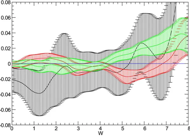
be kept is large. We would like to examine the accuracy and the cost in calcu-lations of GF,η

(

ω, ;T εS,Nsm

)

. In Figure 1, we show our numerical results of

(

)

, , ; ,

F S sm

G _η ωT ε N on the lattice N=20 with 1T =1.60, k=

(

2π 5, π 5

)

and ε =0.5 as a function of

ω

. In this figure we plot the difference

(

; ,

)

F S sm

D ω ε N given by

(

; ,

)

,

(

, ; ,

)

(

,

)

F S sm F S sm F

D ω ε N =G _η ω T ε N −G ω T (37)

The error bar is the statistical error of GF,η

(

ω, ;T εS,Nsm

)

. Compared with

the black data

(

ε =S 0.08,Nsm=40

)

, the green data

(

ε =S 0.08,Nsm =720

)

,

are closer to zero. In comparison with the black data and the red data:

(

ε =S 0.02,Nsm=40

)

, the latters are closer to zero. The average numbers of

the basis states with non-zero coefficients in the SSS method are ~9500 with

0.08 S

ε = _{and ~37000 with} ε =S 0.02. In section 3 we have argued that the

average number of the basis states with non-zero coefficients is drastically

reduced to be of order of NV

ε

S by the SSS method. We see that the mea-

sured values are a little less than NV

ε

S , which are 12500 for ε =S 0.08

and 51200 for ε =S 0.02.

As for the accuracy of sample average, we have discussed that it would be proportional to

ε

S Nsm . Figure 1 shows that the error around ω =3.0 is

~ 0.04 in the black data, ~ 0.01 in the red data and ~ 0.01 in the green data. Since {

ε

S Nsm (black data)}/{

ε

S Nsm (red data)} = 4 ~ 0.04/0.01 and

{

ε

S Nsm (black data)}/{

ε

S Nsm (green data)} = 18∼0.04 0.01, these

[image:9.595.210.536.430.664.2]

results support the discussion in section 3.

Figure 1. The difference DF

(

ω ε; S,Nsm

)

defined in (37) in the SSS method on the

20

(10)

In order to examine GR

(

ω, ;T NR

)

using the SSS method, we define

(

)

, , ; ,

R R S

G η ωT N ε by

(

)

( ) ( ) ( ) ( )

( )

( ) ( )

(

)

(

)

1 2

,

† †

1 1

,1 ,1 , ,

1 , 1 , 1

†

2

, , 2

, ,

, ; , 1

2

ˆ ₀ _;

R

R R S

N M M

r r

F Br i j i k j k

r i j k k

R

k k R R

r r r r

j i

G T N

C C a b a b

N

A Z N

E E

η

η η

φ ψ

ω ε

ε

ψ φ β

ω ε

− −

= = =

 =  

 

× 

 ₋ ₋ ₊ _{ }

 _{ }

  

∑

(38)

(

)

ˆ

1 1 ;

R

N

H

R R r r

r R

Z N R e R

N

β

β −

=

∑

₍₃₉₎

Note that here we set Nsm=1 because one sampling for each random set

will be enough when NR is large. Further discussion on this point will be

given in the final section.

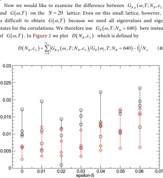
Now we would like to examine the difference between GR,η

(

ω, ;T NR,εS

)

and G

(

ω,T

)

on the

N

=

20

lattice. Even on this small lattice, however, it

is difficult to obtain G

(

ω,T

)

because we need all eigenvalues and eigen

states for the correlations. We therefore use GR

(

ω, ;T NR =640

)

here instead

of G

(

ω,T

)

. In Figure 2 we plot D N

(

R,εS

)

which is defined by

(

)

,

(

)

(

)

0

, , ; , , ; 640 1

N

R S R i R S R i R

i

D N G T N G T N N

ω

η ω

ε ω ε ω

=

[image:10.595.209.533.289.642.2]

=

∑

= − ₍₄₀₎

Figure 2. The difference D N

(

_R,ε_S

)

defined in (40) in the SSS method on the N=20 lattice with 1T =1.60 and k=

(

2π 5,π 5

)

. For each ε_S we present four D N

(

_R,ε_S

)

calculated by four sets of

{

R1 ,R2 ,, RNR

}

. They are plotted by black circles

(

N_R=64

)

and by red circles

(

N_R=256

)

. Results of ε_S=0 are obtained without

(11)

where ωi= × ∆i ω, 0.0625∆ =ω , and Nω =120. In order to examine the

fluctuation of GR,η

(

ω, ;T NR,εS

)

due to the sampling, we carry out

calcula-tions with four sets of

{

R1 , R2 ,, RN_R

}

for each εS. The observed four

(

R, S

)

D N ε are plotted by the black circles

(

NR =64

)

and the red diamonds

(

NR=256

)

. In Figure 2 we also plot results for D N

(

R,ε =S 0

)

, which are

obtained without using the SSS method. Note that they should give us the minimum of the accuracy for D N

(

R,ε ≠S 0

)

. For both cases of NR =64 and

256 R

N = we observe that D N

(

R,ε ≠S 0

)

and D N

(

R,ε =S 0

)

are almost

the same order for any value of εS we employed. This fact implies that in

calculations of the dynamical correlations using the SSS method we do not need more number of the sampling compared to that without the SSS. By these examinations we conclude that we can apply the SSS method to calcula-tions of the dynamical correlacalcula-tions.

5. Higgs Mode

The most important purpose of this paper is the numerical verification of the Higgs mode in the quantum spin systems at finite temperature. In this section we would like to show it by calculating the dynamical correlations in the spin- 1/2 Heisenberg antiferromagnet on the square lattice. Since the Higgs mode is the excited state and couples to the two Goldstone-Nambu modes, we have to calculate the dynamical correlations of the two operators that contain the Gold-stone-Nambu modes. In the Heisenberg antiferromagnet the spin operators contain these modes. Therefore we calculate the following dynamical correlation,

(

)

, , ; ,

R R S

G η ω T N ε in (39) with the two spin operators

( )

( ) ( )

ˆ ₀ ˆ ₀ _ˆz _ˆz

A =B =s k s −k .

In order to obtain stable results at any temperature, we employ the Chebyshev polynomial expansion [39] for the calculation of Hˆ 2

r

e−β R in (7) and (9),

(

)

(

)

ˆ 2

1

ˆ 2

Nc H

r k k c r

k

e−β R p β T H h R

=

∑

(41)

with the k-th Chebyshev polynomial Tk

( )

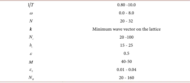
x and the k-th coefficient pk.

[image:11.595.208.539.590.735.2]

Before presenting our results we comment on parameters in our calculations, which we summarize in Table 1.

Table 1. Parameters of calculations; the symbol and the range in our calculations.

1T 0.80 -10.0

ω 0.0 - 8.0

N 20 - 32

k Minimum wave vector on the lattice

c

N 20 -100

c

h 15 - 25

ε 0.5

M 40-50

S

ε _{0.01 - 0.04}

R

(12)

The inverse temperature β =1T and the energy ω are the physical

quan-tities.

The lattice size

N

is restricted because of the exact diagonalization

ap-proach.

In our work, we calculate on the lattices of the size

20 ≤ ≤

N

32

. For the

pe-riodic boundary condition we have two edge vectors

(

l11,l12

)

and

(

l21,l22

)

. Since we impose the π 2 rotational symmetry to the Hamiltonian, the edge vector

(

l21,l22

)

is given by

(

−l12,l11

)

and the lattice size is given by

2 2

11 12

N =l +l .

Note that these edge vectors are defined uniquely for a given lattice size

N

ex-cept for an accidental case

N

=

25

. In this exceptional case we distinguish two

different

N

=

25

lattices by

25 a

and

25 b

. For the lattices of

20, 25 , 25 , 26, 29

N = a b and 32, the edge vector

(

l11,l12

)

are (4, 2), (5, 0), (4, 3), (5, 1), (5, 2) and (4, 4), respectively.

The wave vector

k

is the non-zero wave vector of the lowest magnitude on

the each lattice. For the lattices N=20, 25 , 25 , 26, 29a b and 32, they are

(

2π 5, π 5 , 2π 5,0 , 8π 25,6π 25 , 5π 13, π 13 , 10π 29,4π 29

) (

)

and

(

π 4, π 4

)

.

The parameters Nc and hc control the accuracy of the Chebyshev

poly-nomial expansion. They are determined by the request that the precision is of

order 12

10− . As a result they depend on values of

N

and T.

On the parameter ε_{in (14), we have presented the careful discussion in the}

previous work [29]. This discussion has showed that

ε =

0.5

is most suitable.

Therefore we use this value for ε_.

As for the number M of the Lanczos states we fix it to be 50 following the

discussion of the previous work [29] and the preliminary study. In the

N

=

32

lattice we use

M

=

40

in order to reduce a huge calculation time.

We apply the SSS method to calculations for

N

≥

25

. The parameter εS is

0.01 for N=25 , 25 , 26a b and 29, and is 0.04 for

N

=

32

.

The sampling number of the random states NR is determined by requiring

that the relative precision of our calculations on the dynamical correlations is 5%.

In Figure 3 we present the dynamical correlations GR,η

(

ω, ;T NR,εS

)

on the

29 N

=

lattice as a function of ω. At the low temperatures 1T=10.0, 6.4

and 3.2 we find the broad peaks clearly, as expected. These broad peaks could be the Higgs mode which has been found at

T

=

0

in the previous work [29]. On

the other hand, at the high temperature 1T =1.2 we cannot find any peak that

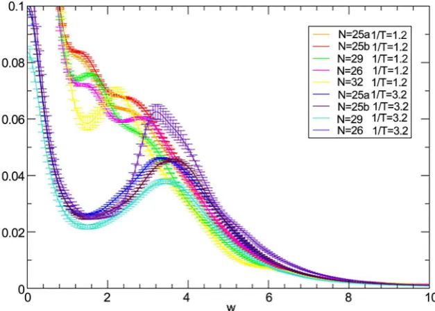
is relevant with the Higgs mode. In order to confirm that we find the broad peak at the low T in the contrast to no broad peak at high T, we plot the dynamical

correlations at the low T and those at the high T on various lattices in Figure

4, where the correlations at 1T =3.2 and those at 1T =1.2 are shown. The

results in Figure 4 support our arguments.

What we are interested in is the shape of the dynamical correlation around the broad peak. Since the absolute value of the correlation strongly depends on T,

(13)

[image:13.595.213.536.69.263.2]

Figure 3. The dynamical correlations GR,η

(

ω, ;T NR,εS

)

on the N=29 lattice for various values of T. They are plotted as a function of ω. The error bars are the statistical errors. The vertical red solid-line shows the value of ω_c. The vertical violet

dashed-lines show the value of ω_c± Γ2 .

Figure 4. The dynamical correlations with 1T=3.2 and 1.2 for various lattices plotted

as a function of ω. The error bars are the statistical errors.

(

)

(

)

, , ; , , , ; ,

R R S R R S

S _η ω T N ε =G _η ω T N ε C (42)

(

)

, , ; , U

i L

R i R S

C G T N

ω η ω ω

ω ε ω

=

∑

∆ ₍₄₃₎

, 0.0625

i L i

ω ω= + × ∆ω ∆ =ω (44)

in the range ωL< <ω ωU which covers the area of the broad peak at

T

=

0

, so

that we can easily compare our results for the different values of T. We employ

2

L c

[image:13.595.213.527.348.572.2]

(14)

c

ω and the width Γ_at

T

=

0

[29]. In Figure 5 we plot SR,η

(

ω, ;T NR,εS

)

on the

N

=

25 a

lattice as a function of ω for various values of 1T between

1.12 and 10.0. We see that the broad peak gradually disappears as 1T becomes

small. For example we can clearly find the broad peak at 1T =3.20, while it is

not easy to find the peak when 1T=1.44 and there is no peak at 1T =1.20.

We would like to determine a boundary of 1T below which the broad peak

vanishes. It is, however, difficult to estimate such boundary temperature because the broad peak disappears gradually when 1T decreases. Therefore we

intro-duce two kinds of T, which we denote Ts and Tl. We can insist that the

broad peak exists for T≤Ts. On the other hand we admit that it is difficult to

find the broad peak for T≥Tl. In other words Ts is a boundary by the strict

condition for the broad peak, while Tl is a boundary by the loose condition for

it. On the

N

=

25 a

lattice we estimate that 1Ts=2.24 and 1Tl =1.76.

On other lattices we can determine Ts and Tl in the same way. When the

lattice size

N

is odd we observe that 1Ts and 1Tl scarcely depend on

N

.

In Figure 6 we show the normalized correlations SR,η

(

ω, ;T NR,εS

)

for 1Ts

and those for 1Tl on the N=25 , 25a b and 29 lattices. On the even-size

lat-tices of

N

=

20, 26

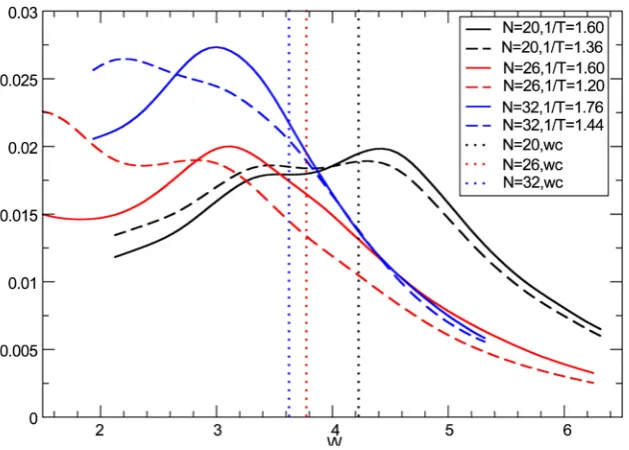
and 32, on the contrary, the shapes differ from each other.

As a result we cannot determine a common value for 1Ts or 1Tl. Our

esti-mations are 1Ts=1.60, 1Tl =1.36 for the

N

=

20

lattice, 1Ts=1.60, 1Tl=1.20 for the

N

=

26

lattice and 1Ts=1.76, 1Tl =1.44 for the

32 N

=

lattice. In Figure 7 we plot the normalized correlations for 1Ts and

those for 1Tl on the

N

=

20, 26

and 32 lattices.

Such difference between the results on the odd-size lattices and those on the even-size lattices is ascribable to the behavior of the correlations at

T

=

0

[29].

[image:14.595.213.532.473.700.2]

As shown in Figure 6 and Figure 7, values of ωc fluctuate more on the even-

(15)

[image:15.595.216.531.66.298.2]

Figure 6. The dynamical correlations for Ts and Tl on the odd-size lattices. The vertical dotted lines show the values of ωc.

Figure 7. The dynamical correlations for Ts and Tl on the even-size lattices. The vertical dotted lines show the values of ωc.

size lattices than those on the odd-size lattices. Especially we observe that

(

20

)

(

26, 32

)

c N c N

ω = ω = . As for the height of the broad peak, it becomes

large when the width Γ is small because the normalization factor

C

in (42) is

calculated in the range between ω − Γc 2 and ω + Γc 2 . Values of the width we

calculated are Γ

(

N =25a

)

=1.41, 25Γ

(

N= b

)

=1.09, and Γ

(

N=29

)

=1.18,

while Γ

(

N=20

)

=1.06, 26Γ

(

N=

)

=1.24, and Γ

(

N=32

)

=0.86.

[image:15.595.212.527.353.578.2]

(16)

different from those on larger lattices. It seems to be that the finite size effect is quite severe for this lattice size. Except for the

N

=

20

case we see the position

of the broad peak shifts to lower ω when

T

>

0

, for which the Higgs mode

with the total spin

J

>

0

should contribute in addition to the mode with

J

=

0

.

6. Summary and Discussion

In this research we have calculated, in order to find the Higgs mode, the dynam-ical correlations of the two spin operators in the spin-1/2 Heisenberg antiferro-magnet on the square lattice at finite temperature. We have proposed an im-proved finite temperature Lanczos method using the stochastic state selection method for calculations on the lattices of up to 32 sites.

In the standard finite temperature Lanczos method we generate Lanczos states, calculate the eigenvalues and calculate matrix elements that are the values of the operator between two Lanczos states. In calculations of the matrix elements we have to keep the set of Lanczos states on the computer memory. Therefore the memory limits the system size for which we can calculate the matrix elements. Here we have proposed the application of the stochastic state selection method in order to weaken this limitation. This method is to select some parts of basis states stochastically and to abandon other basis states. Only by the selected basis states we calculate the inner product. After we make the statistical average, we can obtain the correct value of the inner product. By the stochastic state selec-tion method we can drastically reduce the number of the basis states for the cal-culations.

In order to study the Higgs mode at finite temperature, we have calculated the dynamical correlations of the two spin operators in the spin-1/2 Heisenberg an-tiferromagnet on the square lattice, using the improved finite temperature Lanczos method. In calculations on the

N

=

20 ~ 32

lattices we have found the

broad peaks at low T, while there have been no peaks relevant with the Higgs

mode at high T. Also we have found that the broad peak disappears gradually

in the range 1.76<1T<2.24 on the odd-size lattices, and it disappears

gradu-ally in the range 1.20<1T<1.76 on the even-size lattices.

A few comments are in order. The first comment is about the parameter M

of the Lanczos state number. In the present calculations we used the value of

50 M

=

. At quite high temperature we need the larger value of M, because

many states contribute to the correlations. In a case of

N

=

20

and 1T=0.40,

for an example, we find that the curve of the dynamical correlations vibrates

when

M

=

50

whereas we find the smooth curve when

M

=

100

. We

con-clude that the vibration is unphysical and originates from the smallness of M.

The second comment is about Nsm, i.e. about the number of the sampling on

the probability variables in the SSS method. In our calculations we have two kinds of the sampling, that are the sampling on the random state and the sam-pling on the SSS variables. In calculations of GR,η

(

ω, ;T NR,εS

)

in (39), we set

1 sm

N = . It is possible to obtain the correct values of GR

(

ω,T

)

when we make

(17)

the probability variables

η

by large Nsm for each random state. But it is also

possible to make the sampling on the probability variables

η

and the sampling on the random state at the same time. This sampling means that we make one sampling on the probability variables of

η

, i.e. Nsm =1, for each random state

R . Adopting this sampling method, we can obtain the correct values of

(

,

)

R

G ωT if we make the sampling by large NR. The discussion on Nsm =1

was made in the study of the SSS method [43] extensively.

The following three comments are about subjects for future study to be pur-sued. Since we employ the exact diagonalization approaches, the lattice size is severely limited even in the improved FTLM. Therefore it is desirable to make further study by other calculation methods, the high temperature expansions for example, which do not depend on the lattice size.

The results of this work and the previous work [29] suggest that one can find the Higgs mode in experiments of the quantum antiferromagnet on the square lattice if we measure the dynamical correlations of the two spin operators.

Another subject is about universality of the Higgs mode in the quantum spin systems. On the universality study the system on the triangle lattice is quite in-teresting because this system has the three kinds of the Nambu-Goldstone mod-es, whereas the system on the square lattice has the two kinds. It means that there must be an essential difference between both systems. Therefore it is very important to ask about what is the difference between the Higgs modes in these systems.

Acknowledgements

T. M. would like to thank Dr. Yasuko Munehisa for critical reading of the ma-nuscript and for useful discussions.

References

[1] Higgs, P.W. (1964) Broken Symmetries, Massless Particles and Gauge Fields. Phys-ics Letter, 12, 132-133. https://doi.org/10.1016/0031-9163(64)91136-9

[2] Aad, G., et al. (2012) Observation of a New Particle in the Search for the Standard Model Higgs Boson with the ATLAS detector at the LHC. Physics Letters B, 716, 1-29. https://doi.org/10.1016/j.physletb.2012.08.020

[3] Chatrchyan, S., et al. (2012) Observation of a New Boson at a Mass of 125 GeV with the CMS Experiment at the LHC. Physics Letters B, 716, 30-61.

https://doi.org/10.1016/j.physletb.2012.08.021

[4] Pekker, D. and Varma, C.M. (2015) Amplitude/Higgs Modes in Condensed Matter Physics. Annual Review of Condensed Matter Physics, 6, 269-297.

https://doi.org/10.1146/annurev-conmatphys-031214-014350

[5] Endres, M., Fukuhara, T., Pekker, D., Cheneau, M., Schaub, P., Gross, C., Demler, E., Kuhr, S. and Bloch, I. (2012) The “Higgs” Amplitude Mode at the Two-Dimen- sional Super Fluid/Mott Insulator Transition. Nature, 487, 454-458.

https://doi.org/10.1038/nature11255

(18)

Review Letters, 100, Article ID: 205701.

https://doi.org/10.1103/physrevlett.100.205701

[7] Matsunaga, R., Hamada, Y., Makise, K., Uzawa, Y., Terai, H., Wang, Z. and Shima-no, R. (2013) Higgs Amplitude Mode in the BCS Superconductors Nb1-xTixN In-ducedby Terahertz Pulse Excitation. Physical Review Letters, 111, Article ID: 057002. https://doi.org/10.1103/PhysRevLett.111.057002

[8] Measson, M.-A., Gallais, Y., Cazayous, M., Clair, B., Rodiere, P., Cario, L. and Sa-cuto, A. (2014) Amplitude Higgs mode in the 2H-NbSe2 superconductor. Physical Review B, 89, Article ID: 060503. https://doi.org/10.1103/PhysRevB.89.060503

[9] Bjerlin, J., Reimann, S.M. and Bruun, G.M. (2016) Few-Body Precursor of the Higgs Mode in a Fermi Gas. Physical Review Letters, 116, Article ID: 155302.

[10] Grenier, B., Petit, S., Simonet, V., Canevet, E., Regnault, L-P., Raymond, S., Canals, B., Berthier, C. and Lejay, P. (2015) Longitudinal and Transverse Zeeman Ladders in the Ising-Like Chain Antiferromagnet. Physical Review Letters, 114, Article ID: 017201. https://doi.org/10.1103/PhysRevLett.114.017201

[11] Kemper, A.F., Sentef, M.A., Moritz, B., Freericks, J.K. and Devereaux, T.P. (2015) Direct Observation of Higgs Mode Oscillations in the Pump-Probe Photoemission Spectra of Electron-Phonon Mediated Superconductors. Physical Review B, 92, Ar-ticle ID: 224517. https://doi.org/10.1103/physrevb.92.224517

[12] Sherman, D., Pracht, U.S., Gorshunov, B., Poran, S., Jesudasan, J., Chand, M., Ray-chaudhuri, P., Swanson, M., Trivedi, N., Auerbach, A., Scheffler, M., Frydman, A. and Dressel, M. (2015) The Higgs Mode in Disordered Superconductors Close to a Quantum Phase Transition. Nature Physics, 11, 188-192.

https://doi.org/10.1038/nphys3227

[13] Podolsky, D., Auerbach, A. and Arovas, D. (2011) Visibility of the Amplitude (Higgs) Mode in Condensed Matter. Physical Review B, 84, Article ID: 174522.

https://doi.org/10.1103/physrevb.84.174522

[14] Barlas, Y. and Varma, C.M. (2013) Amplitude or Higgs Modes in D-Wave Super-conductors. Physical Review B, 87, Article ID: 054503.

https://doi.org/10.1103/PhysRevB.87.054503

[15] Tsuchiya, S., Ganesh, R. and Nikuni, T. (2013) Higgs Mode in a Superfluid of Dirac Fermions. Physical Review B, 88, Article ID: 014527.

[16] Liu, B., Zhai, H. and Zhang, S. (2016) Evolution of the Higgs Mode in a Fermion Superfluid with Tunable Interactions. Physical Review A, 93, Article ID: 033641.

https://doi.org/10.1103/physreva.93.033641

[17] Nakayama, T., Danshita, I., Nikuni, T. and Tsuchiya, S. (2015) Fano Resonance through Higgs Bound States in Tunneling of Nambu-Goldstone Modes. Physical Review A, 92, Article ID: 043610. https://doi.org/10.1103/physreva.92.043610

[18] Weidinger, S.A. and Zwerger, W. (2015) Higgs Mode and Magnon Interactions in 2D Quantum Antiferromagnets from Raman Scattering. European Physical Journal B, 88, 237. https://doi.org/10.1140/epjb/e2015-60438-1

[19] Bruun, G.M. (2014) Long-Lived Higgs Mode in a Two-Dimensional Confined Fer-mi System. Physical Review A, 90, Article ID: 023621.

https://doi.org/10.1103/physreva.90.023621

(19)

[21] Xian, Y. and Merdan, M. (2014) Longitudinal Excitations in Bipartite and Hex-agonal Antiferromagnetic Spin Lattices. Journal of Physics: Conference Series, 529, Article ID: 012020. https://doi.org/10.1088/1742-6596/529/1/012020

[22] Yi-Xiang, Y., Ye, J. and Liu, W.-M. (2013) Goldstone and Higgs Modes of Photons inside a Cavity. Scientific Report, 3, 3476.

[23] Gazit, S., Podolsky, D., Auerbach, A. and Arovas, D. (2013) Dynamics and Conduc-tivity near Quantum Criticality. Physical Review B, 88, Article ID: 235108.

[24] Rancon, A. and Dupuis, N. (2014) Higgs Amplitude Mode in the Vicinity of a (2+1)-Dimensional Quantum Critical Point. Physical Review B, 89, Article ID: 180501. https://doi.org/10.1103/PhysRevB.89.180501

[25] Gazit, S., Podolsky, D. and Auerbach, A. (2013) Fate of the Higgs Mode near Quantum Criticality. Physical Review Letters, 110, Article ID: 140401.

[26] Katan, Y.T. and Podolsky, D. (2015) Spectral Function of the Higgs Mode in 4-ε

Dimensions. Physical Review B, 91, Article ID: 075132.

[27] Rose, F., Leonard, F. and Dupuis, B. (2015) Higgs Amplitude Mode in the Vicinity of a (2+1)-Dimensional Quantum Critical Point: A Nonperturbative Renormaliza-tion-Group Approach. Physical Review B, 91, Article ID: 224501.

[28] Nishiyama, Y. (2015) Critical Behavior of the Higgs- and Goldstone-Mass Gaps for the Two-Dimensional S=1 XY Model. Nuclear Physics B, 897, 555-562.

https://doi.org/10.1016/j.nuclphysb.2015.06.006

[29] Munehisa, T. (2015) Numerical Study of the Higgs Mode in the Heisenberg Anti-ferromagnet on the Square Lattice. World Journal of Condensed Matter Physics, 5, 261-274. https://doi.org/10.4236/wjcmp.2015.54027

[30] Hatano, N. and Suzuki, M. (1993) Quantum Monte Carlo Methods in Condensed Matter Physics. World Scientific, Singapore, 13-47.

https://doi.org/10.1142/9789814503815_0002

[31] De Raedt, H. and von der Linden, W. (1995) The Monte Carlo Method in Con-densed Matter Physics. Springer, Berlin, 249-284.

[32] Richter, J., Schulenburg, J. and Honecker, A. (2004) Quantum Magnetism. In: Schollwock, U., Richter, J., Farnell, D.J.J. and Bishop, R.F., Eds., An Introduction to Quantum Spin Systems, Springer, Berlin, 135-152.

[33] Auerbach, A. (1994) Interacting Electrons and Quantum Magnetism. Springer, Ber-lin.

[34] Jaklic, J. and Prelpvsek, P. (1994) Lanczos Method for the Calculation of Fi-nite-Temperature Quantities in Correlated Systems. Physical Review B, 49, 5065- 5068. https://doi.org/10.1103/PhysRevB.49.5065

[35] Long, M.W., Prelovsek, P., El Shawish, S., Karadamoglou, J. and Zotos, X. (2003) Finite-Temperature Dynamical Correlation Using the Microcanonical Ensemble and the Lanczos Algorithm. Physical Review B, 68, Article ID: 235106.

[36] Jaklic, J. and Prelpvsek, P. (2000) Finite-Temperature Properties of Doped Antifer-romagnets. Advance Physics, 49, 1-92. https://doi.org/10.1080/000187300243381

(20)

[38] Hanebaum, O. and Schnack, J. (2014) Advanced Finite-Temperature Lanczos Me-thod for Anisotropic Spin Systems. European Physical Journal B, 87, 194.

https://doi.org/10.1140/epjb/e2014-50360-5

[39] Munehisa, T. (2014) An Improved Finite Temperature Lanczos Method and Its Ap-plication to the Spin-1/2Heisenberg Model on the Kagome Lattice. World Journal of Condensed Matter Physics, 4, 134-140. https://doi.org/10.4236/wjcmp.2014.43018

[40] Munehisa, T. and Munehisa, Y. (2003) A New Approach to Stochastic State Selec-tions in Quantum Spin Systems. Journal of the Physical Society of Japan, 72, 2759-2765. https://doi.org/10.1143/JPSJ.72.2759

[41] Munehisa, T. and Munehisa, Y. (2004) The Stochastic State Selection Method for Energy Eigenvalues in the Shastry-Sutherland Model. Journal of the Physical Society of Japan, 73, 340-347. https://doi.org/10.1143/JPSJ.73.340

[42] Munehisa, T. and Munehisa, Y. (2004) Numerical Study for an Equilibrium in the Recursive Stochastic State SelectionMethod. arXiv: cond-mat, 0403626.

[43] Munehisa, T. and Munehisa, Y. (2004) A Recursive Method of the Stochastic State Selection for Quantum Spin Systems. Journal of the Physical Society of Japan, 73, 2245-2251. https://doi.org/10.1143/JPSJ.73.2245

[44] Munehisa, T. and Munehisa, Y. (2006) The Stochastic State Selection Method Com-bined with the Lanczos Approachto Eigenvalues in Quantum Spin Systems. Journal of Physics: Condensed Matter, 18, 2327-2335.

https://doi.org/10.1088/0953-8984/18/7/018

[45] Munehisa, T. and Munehisa, Y. (2007) An Equilibrium for Frustrated Quantum Spin Systems in the Stochastic State Selection Method. Journal of Physics: Con-densed Matter, 19, Article ID: 196202.

https://doi.org/10.1088/0953-8984/19/19/196202

[46] Munehisa, T. and Munehisa, Y. (2009) A Constrained Stochastic State Selection Method Applied to Frustrated Quantum Spin Systems. Journal of Physics: Con-densed Matter, 21, Article ID: 236008.

https://doi.org/10.1088/0953-8984/21/23/236008

[47] Munehisa, T. and Munehisa, Y. (2010) Numerical Study of the Spin-1/2 Heisenberg Antiferromagnet on a 48-Site Triangularlattice Using the Stochastic State Selection Method. arXiv, 1081161.

[48] Hams, A. and De Raedt, H. (2000) Fast Algorithm for Finding the Eigenvalue Dis-tribution of Very Large Matrices. Physical Review E, 62, 4365-4377.

https://doi.org/10.1103/PhysRevE.62.4365

[49] Iitaka, T. and Ebisuzaki, T. (2004) Random Phase Vector for Calculatingthe Trace of a Large Matrix. Physical Review E, 69, Article ID: 057701.

(21)

Submit or recommend next manuscript to SCIRP and we will provide best service for you:

Accepting pre-submission inquiries through Email, Facebook, LinkedIn, Twitter, etc. A wide selection of journals (inclusive of 9 subjects, more than 200 journals)

Providing 24-hour high-quality service User-friendly online submission system Fair and swift peer-review system

Efficient typesetting and proofreading procedure

Display of the result of downloads and visits, as well as the number of cited articles Maximum dissemination of your research work

Submit your manuscript at: http://papersubmission.scirp.org/