9
Robust Controller Design using Quantitative Feedback
Theory (QFT)
Vilas.K Jadhav
Lecturer, Instrumentation &Control
Engineering Department
Pravara Rural Engineering College
Loni
Chandrakant.B Kadu
Assistant Professor, Instrumentation
&Control Engineering Department
Pravara Rural Engineering College.
Loni
Bhagsen.J.Parvat
Assistant Professor,
Instrumentation &Control
Engineering Department
Pravara Rural Engineering
College. Loni
ABSTRACT
Most of the practical systems are characterized by high uncertainty which makes it difficult to maintain good stability margins and performance properties for closed loop system. In case of conventional control, if plant parameter changes we cannot assure about the system performance hence it is necessary to design robust control for uncertain plant. Among the various strategies proposed to tackle this problem, Quantitative Feedback Theory (QFT) has proved its superiority especially in the face of significant parametric uncertainty. The feature of QFT is that it can take care of large parametric uncertainty along with phase information. For the purpose of QFT, the feedback system is normally described by the two-degrees-of freedom structure. A chemical system common to many chemical processing plants, known as a continuous stirred tank reactor (CSTR).For an isothermal CSTR the product concentration can be controlled by manipulating the feed flow rate,which changes the residence time.
Keywords—
Robust Control, PID Control, Continuous stirred tank reactor, Quantitative Feedback Theory (QFT).
1.INTRODUCTION
PID controllers have dominated the process control industry over the decades owing to its associated simplicity and easiness in implementation. The needs for better control strategies for process control in order to achieve better performance have always motivated research interests. The design of PID controllers, tuning involves selecting the amounts of Proportional, Integral and Derivative components required at the output of the controller. Since the design of PID controllers involves obtaining the P, I and D components there always occur a compromise in the design. The design of the optimum values for the PID controller parameters has always been challenging. Many new tuning techniques have been developed for the design of PID controllers, however then still exists a scope for better tuning method. Various control strategies are used for design of control system depending on plant model [1].
If the design performs well for substantial variations in the dynamics of the plant from the design values, then the design is robust. Robust control deals explicitly with uncertainty in its approach to controller design. Quantitative Feedback Theory (QFT) is robust control method which deals with the effects of uncertainty systematically. QFT is a graphical loop shaping procedure used for the control design of either SISO (Single Input Single Output) or MIMO (Multiple Input Multiple Output) uncertain systems including the nonlinear
And time varying cases. QFT [5],[7],developed by Isaac Horowitz is a frequency domain technique utilizing the Nichols chart (NC)
in order to achieve a desired robust design over a specified region of plant uncertainty. In comparison to other robust control methods, QFT offers a number of advantages. For the purpose of QFT, the feedback system is normally described by the
two-degrees-of freedom structure. A
proportional–integral–derivative controller (PID controller) is a generic control loop feedback mechanism widely used in industrial control systems. A PID controller attempts to correct the error between a measured process variable and a desired set-point by calculating and then outputting a corrective action that can adjust the process accordingly. A chemical system common to many chemical processing plants, known as a continuous stirred tank reactor (CSTR) for an isothermal CSTR the product concentration can be controlled by manipulating the feed flow rate,which changes the residence time.
2.
BASICS
OF
PID
CONTROL
SYSTEM
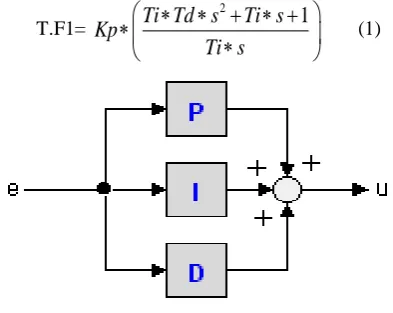
A PID controller consists of the three terms: proportional (P), integral (I), and derivative (D). Its behavior can be roughly interpreted as the sum of the three term actions The P term gives a rapid control response and a possible steady state error, the I term eliminates the steady state error and the D term improves the behavior of the control system during transients.
2.1
Parallel Form
It can be seen that P, I and D channels react on the error signal and that they are unbundled [3],[4].
T.F1=
2
1
Ti Td s
Ti s
Kp
Ti s
[image:1.595.324.521.541.697.2]
(1)
10
A PID controller in series form (also known as interacting
Form), has the control equation.
1
(1
)(1
)
u
kp
Tds e
Tis
(2)
The controller actions (P, I and D) act dependently as can be
[image:2.595.306.511.150.308.2]seen in the corresponding block diagram representation
Fig.2: Series form of PID
T.F2=
*(1
1
) *(1
*
)
*
kp
s Td
Ti s
(3)
3. QFT
BASIC
CONCEPTS
QFT is a very powerful control system design method when the plant parameters vary over a broad range of operating conditions. The basic concept of QFT is to define and take into account, along the control design process, the quantitative Relation between the amount of uncertainty to deal with and the amount of control effort to use. The Quantitative Feedback Theory (QFT) method offers, frequency-domain based design approach for tackling feedback control problems with robust performance objectives [2]. In this approach, the plant Dynamics may be described by frequency response data, or by a transfer function with mixed (parametric and nonparametric) Uncertainty models. The basic idea in QFT is to convert design specifications at closed loop and plant uncertainties into robust stability and performance bounds on open loop transmission of nominal system and then design controller by using loop shaping [5].
4.
CONTROLLER
DESIGN
PROCEDURE
Design Steps for PID Controller are as follows [5].
1
Translation of TDS to FDS (Time Domain Specification toFrequency Domain Specification)
2 Generation of the Plant Set.
3 Generation of the Template
4 Selection of Nominal Plant.
5 Generation of Stability Bounds
6 Generation of Tracking Bounds
7 Grouping of Bounds
8 Intersection of Bounds
9 Loop shaping (Design of a Controller)
10 Prefilter Design
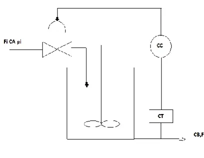
[image:2.595.56.286.190.370.2]A chemical system common to many chemical processing plants, known as a continuous stirred tank reactor (CSTR), was utilised as a suitable test for,TSK Fuzzy control, ANFIS control and PID control.
Fig. 3. CSTR process
It suffices to know that within the CSTR two chemicals are mixed, and react to produce a product compound with concentration. The temperature of the mixture is a schematic representation of the system is shown in Fig. 3 For an isothermal CSTR, the product concentration can be controlled by manipulating the feed flow rate, which changes the residence time (for constant volume reactor).Here we consider the series parallel reaction of the following form
A B C
2A D
The desired product is the component B, the intermediate component in the series reaction. In this module we find the steady state and dynamic behavior that can occur with this reaction scheme. Where A=cyclopentadiene, B=cyclopentenol, C=cyclopentanediol, D=dicyclopentadiene
The molar rate of formation (per unit volume) of each component is Overall material balance is [6]
(
)
d
vp
fi
fp
dt
(4)The liquid phase density is not a function of concentration, vessel liquid outlet density is equal to the inlet steam density, i.e. f=fi, the input output transfer function for the reactor is
( ) 2
1.1170
3.1472
4.6429
5.3821
p S
s
g
s
s
(5)
Performance specifications:
1. Stability Specifications: Gain margin > 5db and Phase
Margin=450
2. Tracking Specifications: 0.9s ≤ rise time≤1.2s and 0%
11
5.1 Design Steps
1. The time domain specifications are translated into Frequency domain. The corresponding transfer functions
For upper and lower specifications are as follows:
2
0.738
13.62
7.38
13.62
RU
s
T
s
s
(6)3 2
113.3
20.94
104.1
113.3
RL
T
s
s
s
(7)It represents the characteristics of plant and desired system performance specifications in frequency domain. In many control systems the output y (t) must be between specified upper and lower bounds, y(t)u and y(t)L, respectively The conventional time-domain figures of merit, based upon a step input signal They
[image:3.595.307.548.63.226.2]are: Mp, peak overshoot;
t
r rise time,t
p peak time andt
s settling time. Corresponding system performance specifications in the frequency domain are, Bu and BL, the upper and lower bounds respectively. Assuming that the control system has negligible sensor noise and sufficient control effort authority, then for a stable linear-time-invariant (LTI) minimum-phase plant a LTI compensator may be designed to achieve the desired control system performance specifications The frequency response of performance specifications are Shown in figure 4Fig 4: Bode plot
5.2 Plant Templates
Templates are plot of magnitude verses phase of plant sets for various frequencies.
Fig 5: Plant Template
Generation of templates at specified frequencies that pictorially describe region of plant parameter uncertainty on the Nichols chart. Which define the structured plant parameter uncertainty.
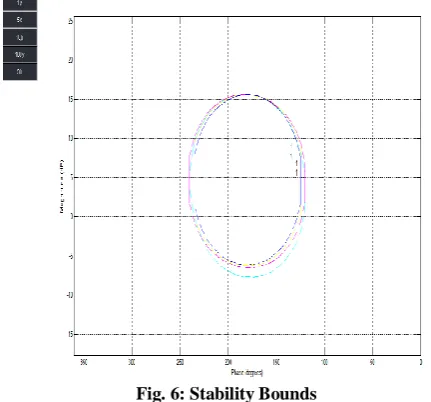
5.3 Stability bounds
[image:3.595.64.287.415.597.2]It is well known that magnitude of T (jw) ≤ ML establishes a circle in the Nichols Chart. The specifications on system performance in the time domain and in the frequency domain identify a minimum damping ratio for the dominant roots of the closed-loop system which corresponds to a bound on the value of Mp =Mm. On the NC this bound on Mp = ML establishes a region which must not be penetrated by the templates and the loop transmission functions for all frequencies. The boundary of this region is referred to as the universal high-frequency boundary (UHFB) or stability bound, the U-contour [5].
Fig. 6: Stability Bounds
5.4 Tracking Bounds
[image:3.595.315.531.441.642.2]12
Fig. 7: Tracking Bounds
5.5 Grouping of bounds
Fig. 8: Grouping of Bounds
5.6 Intersection of Bounds
Fig. 9: Intersection of bounds
[image:4.595.317.530.119.332.2]Loop shaping is a design method where it is attempted to choose a controller such that the loop transfer function obtains the desired shape.
Fig. 10: Loop shaping
It is a key design step and it consists of shaping of the open loop function to set the boundaries given by the design specifications. Manual loop shaping can be done with use of QFT Matlab toolbox. The controller design is undertaken on the NC considering the frequency constraints and the nominal loop L0(s) of the system. At this point, the designer begins to introduce controller functions (G(s)) and tune their parameters, a process called Loop Shaping, until the best possible controller is reached without violation of the frequency constraints the loop shaping with nominal plant is as shown in figure 10.
The controller obtained after loop shaping is
2
0.2129
102.1
3980
( )
s
s
C s
s
(8)
5.8 Filter Design
In order to keep desired tracking performance specifications,
Using Matlab QFT toolbox prefilter is designed
2
1
( )
0.08976
0.7368
1
F s
s
s
[image:4.595.58.256.547.729.2]13
Fig. 11: Prefilter Design
After manual loop shaping we got the QFT elements that is Transfer function of controller If we compare that transfer function with the transfer function of parallel PID controller (eq. 1) we will get the PID parameters. Hence transfer function of controller is
2
0.2129
102.1
3980
( )
s
s
C s
s
(10)
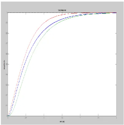
The PID parameters are as follows
Ti=0.02565, Td=0.002085, Kp=102.92
Fig. 12: Step response of all systems.
6. CONCLUSION
In case of conventional control, if plant parameter changes we cannot assure about the system performance hence it is necessary to design robust control for uncertain plant. The modern control systems such as H-2, H∞ and μ-synthesis can’t handle large uncertainty and are applicable to single input single output (SISO) LTI systems. The drawbacks of conventional and modern control theory are eliminated by classical control theory based method which can handle large parameter uncertainty and works in frequency domain called as QFT.We have designed a PID controller using QFT for an industrial application i.e. continuous stirred tank reactor process for specified tracking requirements.
7. REFERENCES
[1] L. J. Nagrath and M. Gopal, “Control Systems Engineering.” New Age International (P) Limited
[2] Joaquin Cervera, Alfonso Banos et al., “Tuning of Fractional PID Controllers by Using QFT”, IEEE, 2006, page no.5402-5406
[3] Graham C.Goodwin, “Control System Design”, Prentice-Hall of India Private Limited.
[4] A. C. Zolotas and G. D. Halikias, “Optimal Design of PID controllers using the QFT method”, IEEE Proceedings, Control Theory Appl., Vol.146, November 1999, page No.585- 589.
[5] C.H.Houpis, “Quantitative Feedback Theory Fundamentals and applications.”Taylor and Francis Group publication, 2006.
[6] B.Wayne Bequette.“Process control modeling design and simulation” Prentice-Hall of India Private Limited, Page no.605-614.
[image:5.595.65.268.477.682.2]