Pixel Dependent Automatic Parameter Selection for
Image Denoising with Bilateral Filter
C. Shyam anand
Dept. of EEE, Indian Institute of Technology Guwahati, Guwahati, Assam, India
J. S. Sahambi
Dept. of EEE, Indian Institute of Technology Guwahati, Guwahati, Assam, India
ABSTRACT
Image denoising using bilateral filter is controlled by the width of its smoothing functions namely the domain and the range components. The choice of the width of range function is image dependent and requires several experiments. This paper presents an automatic method based on power-law scaling of the inverse of local statistics for pixel wise estimation of range parameter. This leads to an adaptive range function that is narrow along the edges and wide for smooth regions. The experimental results validate the performance of the proposed method of parameter selection in denoising images corrupted by additive white Gaussian noise.
General Terms
Image Denoising, Adaptive Bilateral Filter.
Keywords
Automatic parameter selection, bilateral filter, denoising, local statistics, pixel adaptive.
1.
INTRODUCTION
The main objective of the advanced techniques in image denoising is to preserve the structural details while removing the noise. This is achieved by employing locally adaptive nonlinear filters that depend on the image characteristics. The adaptive filtering limits smoothing along the edges and thus reduces blurring. Therefore, these can also be referred as edge-preserving adaptive filters.
Methods like anisotropic diffusion, weighted least squares and robust statistics are among the iterative procedures for adaptive filtering of noise [1]. The bilateral filter originally developed by Tomasi et al [2] is a non-iterative method and it gives qualitatively better results than the iterative methods [3]. However, Elad [1] and Barash [4] have shown that bilateral filter and other adaptive filters are fundamentally related. Therefore, the simplicity and flexibility of bilateral filters extends its application in various contexts such as image denoising, contrast enhancement, super resolution, etc [3, 5, and 6].
The bilateral filter consists of two Gaussian weighting functions defined as the domain and the range component. The domain component characterizes the spatial distance and the range component signifies the intensity differences between the pixels defined within a neighbourhood. Basically, the performance of bilateral filter depends on the choice of the width of its smoothing kernels. In previous works [1–4, 7, 8], the widths of the smoothing kernels are chosen experimentally to suit the application. It is also shown that the range component is more decisive than the domain component and its width should be adapted to the noise level for better denoising [7–10].
Liu et al [7] adapted the width of the range kernel to local noise variance estimates for improving the denoising efficiency of bilateral filter and is chosen as 1.95 times of the local noise level. Zhang [8] studied the optimal choice of kernel widths as a function of noise variance. It is verified that the optimal width of range kernel is linearly related to the noise level and is chosen as 1.7 times of the global noise variance. Wong [9] proposed a method to adaptively vary the parameters of bilateral filter based on the local phase characteristics of the image to be denoised. As a result, smoothing in the high contrast regions is limited relative to the smooth regions. However, it requires the range of the filter parameters to be determined experimentally similar to the standard bilateral filter. Rose et al [11] proposed a method to vary the range parameter of the bilateral filter based on the standard deviation of noise.
In this paper, we address the issues in choosing the width of the range kernel and show that it can be determined automatically from the local statistics of the image. The proposed method results in pixel wise adaptation of the filter width. The experimental results show that the proposed method for automatic and pixel wise estimation of the range filter width gives qualitatively similar and possibly improved results for higher noise levels. The experiments were performed on gray scale and colour images.
The rest of the paper is organized as follows: Section 2 discusses about the bilateral filter parameters and presents the proposed method for automatic and pixel wise parameter selection. In Section 3, the experimental results comparing the performance of the proposed method for denoising various images under various noise levels are discussed in detail. Section 4 concludes the paper stating the advantages and the limitations of the proposed method.
2.
BILATERAL FILTER WITH
AUTOMATIC PARAMETER
SELECTION
Define a 2D discrete image
f
xy of sizeN
N
, such that
x y
,
0,...
N
1
0,...
N
1
. Assume thatxy
f
is corrupted by additive white Gaussian noise of variance2 n
1
ˆ
x d y d( ; , ; )
(
;
)
xy s r ij xy ij
i x d j y d
f
W i x j y W f
f
f
C
(1)Where,
d
is a non-negative integer such that(2
d
1) (2
d
1)
denotes the neighborhood windowsize.
W
s andW
r are the domain and range components respectively and are defined as
2
2 2( ; , ; )
exp
2
ss
i
x
j
y
W i x j y
(2) and 2 2(
;
)
exp
.
2
ij xy r ij xyr
f
f
W f
f
(3)The normalization constant
C
is given as1
.
( ; , ; )
(
;
)
y dx d
s r ij xy
i x d j y d
C
W i x j y W f
f
(4)The parameters
s2and
r2are the variances that specify the width of the domain and range kernels respectively.The optimal performance of the bilateral filter depends on the
choice of
sand
r[8]. Hence, they are considered as the controlling parameters. From the definition in (2) it can be inferred that the domain component is independent of the image content. Its influence depends only on the spatial distance between the pixels and not on their intensity values. Conversely, the range component defined in (3) depends on the intensity values and hence, it decreases the influence ofpixels at
i j
,
when their intensity values differ fromf
xy. This implies that the range component adapts to the structural content of the image and therefore, the extent of filtering ismore influenced by the choice of
r[10]. It can be understood that large noise levels require higher values ofr
and vice-versa. This dependency leads to the proportionality,
r
n. (5)
is the constraint parameter that determines the value ofr
. Large value of
will over smooth the image and small values will not suppress noise properly. Generally, the optimal value of
is chosen experimentally such that there remains a trade-off between image smoothing and its sharpness. However, this approach has the following setbacks.(1) It demands several experiments to obtain an optimal
the image content. But real images almost always violate this assumption.
The noise in smooth regions is perceptually more dominant than in the edges and coarse texture regions. This requires comparatively less smoothing along the edges and the coarse details [12]. This problem can be handled by varying the
control parameter
r(and so
) from pixel to pixel. This is done using the local statistics of the image to be denoised.The local mean (variance) of a pixel
f
xyis computed locally over its neighbourhood of size(2
d
1) (2
d
1)
. The mean of a pixelm
xy is defined as [13]
21
2
1
y d x d
xy ij
i x d j y d
m
f
d
. (6)Similarly the variance of a pixel
2xyis obtained from
2 2 21
2
1
y d x dxy ij xy
i x d j y d
f
m
d
(7)In the case of colour images the variance of a pixel is considered as the average of the variances computed from the RGB components.
The pixels belonging to the high contrast regions such as edges and coarse texture regions have high variance and those belonging to smooth regions have low variance values [12]. Since the objective is to restrict
along the high contrast regions it is assumed that
(
xy)
xyxy
max
(8)The locally computed variance varies directly as its mean and so there exists large variations in the value of
corresponding to pixels in the low and high contrast regions. Hence, power-law transformation is performed to stabilize the dynamic range and scale the values of
[14]. Therefore, thevalue of
r for each pixel at
x y
,
is obtained as
r xy
xy n
. (9)The value of parameter
controls the degree of smoothing. The resultant
r is a matrix of control values that variesaccording to the pixel characteristics and is also properly balanced among the pixels belonging to smooth regions, edges and coarse texture regions. The range component in (3) can therefore be redefined as,
2
2
(
;
)
exp
2(
)
ij xy r ij xy
r xy
f
f
W f
f
. (10)
The noisy image
f
ˆ
is generated by adding white Gaussian noise of variance
n2to the original imagef
and is simulated using MATLAB as follows [15]:
n(
( ))
f
f
randn size f
(11)The value of
n is assumed to lie within the range [0.01− 0.1]. The optimal neighbourhood size for computing the local variance and the response of the filter is experimentallydetermined as
11 11
. The optimal value of domain parameter
s is evaluated as 3. The empirical value ofpower variable
in (9) is estimated as9
n for gray scale images and4
n for color images.The values of the range parameter
r computed for each pixel of the noisy Barbara image is shown in Figure 1(a). Itcan be verified that the
r values corresponding to the edge pixels are less than the pixels in flat regions and also the range parameter value for each edge pixel depends on its strength. This is because the strong edges are less influenced by noise than the weak edges. As a result the variance of the strong edge pixels is high and weak edges are characterized by comparatively low variance values. Thus the degree of smoothing along the strong edges is relatively less than the weak edges.From the experiments it is observed that as the noise level increases the local variance in the flat regions increases substantially than in the edges. This can also be verified from the plot in Figure 1(b). For this reason the slope of the
power-law transformation should decrease for high values of
n. Asa result the range of
rxy
values corresponding to thepixels
f x y
,
in the flat regions will be expanded to ensure sufficient smoothing. Figure 1(c) gives the plot ofcontrol values
rxy
obtained for the local variances shown in Figure 1(b). From these plots it is obvious that forhigh noise levels the increase in range values
rxy
for the edges and coarse texture regions are well regulated. Similarly, the range values for the smooth regions are sufficiently boosted to ensure proper smoothing.The effectiveness of the proposed technique for improving the bilateral filter is validated using the root mean square error (RMSE) and the structural similarity (SSIM) index [16]. The value of SSIM index lies between [-1, 1]. Minimum values of RMSE and large values of SSIM index mean high similarity between the compared images.
The results of parameter selection obtained for the experiments performed on the test images for various noise
levels are given in Table 1. From this it can be understood that
the values of
r (both in fixed and adaptive) increases withthe noise level to ensure sufficient smoothing. In the case of
fixed
r as employed in standard bilateral filter [2]; the increase had to be limited to retain the image sharpness. As a result smoothing in flat region will be compensated.Conversely, the adaptive choice allocates higher
rin theflat regions in spite of limited
r in the edges. Thus it achieves good smoothing and retains image sharpness. Also,for low noise levels the range between
r for edges and flatregions is well controlled, such that there is no excess smoothing.
This improvement is confirmed by comparing the values of quality metrics RMSE and the SSIM index given in Table 2. It can be verified that the proposed adaptive parameter estimation strategy yields better results for most of the test images and is particularly higher for increasing noise levels. In the case of Mandrill image the improvement is not as expected. This is because most of the regions in this image are coarse texture regions. Due to the dependence of the proposed
method on local variance values, the estimated
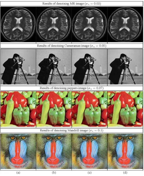
rfor the pixels in these regions were slightly higher. However, the minimal difference in the values of SSIM indicates that the variations will not be perceptually significant. The image denoising results obtained for some of the test images are shown in Figure 2 for visual inspection.4.
CONCLUSSION
This paper presents a simple and intuitive approach for pixel wise adaptation of the smoothing values based on the local variance and thus directs towards automatically tuning the
control parameter
r of the bilateral filter. The experimental results prove that the proposed approach also improves the denoising efficiency of the bilateral filter. This method can be further improved by using adaptive neighborhoods of variable size and shape in order to estimate the local variances and the filter response.The results are presented for noise levels
n
0.1
. However, in the case of
n
0.1
the value of
becomes1
for which the power-law transformation further reduces the value of
xy corresponding to the edge regions. Hence,the level of smoothing along the edges is decreased preserving few noise pixels. This problem limits the advancement of the proposed approach for very low signal to noise ratio images
Figure 1: Results for Barbara image: (a) Illustration of pixel wise allocation of
rvalues for
n
0.05
(b) Plot of local standard deviation
xy estimated for different noise levels. (c) Plot of range parameter values
r estimated corresponding to [image:4.595.56.537.308.499.2]the
xy values in (b).Table 1: Fixed and adaptive range parameter
r estimated for different test images. [a,b] denote the interval of adaptive
r [image:4.595.57.538.540.749.2]Figure 2: Illustration of image denoising results. In column: (a) Original images (b) Noisy images (c) Denoising results using
5.
REFERENCES
[1] M. Elad, “On the Origin of the Bilateral Filter and Ways to Improve it,” IEEE Transaction on Image Processing, vol. 11, no. 10, pp. 1141–1151, October 2002.
[2] C. Tomasi and R. Manduchi, “Bilateral Filtering for Gray and Color Images,” in Proc. 6th Int. Conf. Computer Vision, 1998, pp. 839–846.
[3] S. Paris, P. Kornprobst, J. Tumblin, and F. Durand, Bilateral Filtering: Theory and Applications, Foundations and Trends in Computer Graphics and Vision. Now publishers Inc., 2008, vol. 4, no. 1.
[4] D. Barash, “A Fundamental Relationship between Bilateral Filtering, Adaptive Smoothing, and the Nonlinear Diffusion Equation,” IEEE Transaction on Pattern Analysis and Machine Intelligence, vol. 24, no. 6, pp. 844–847, June 2002.
[5] J.-W. Han, J.-H. Kim, S.-H. Cheon, and J.-O. Kim, “A Novel Image Interpolation Method Using the Bilateral Filter,” IEEE Transactions on Consumer Electronics, vol. 56, no. 1, pp. 175–181, Feb. 2010.
[6] L. Qiegen, L. Jianhua, and Z. Yuemin, “Adaptive Image Decomposition by Improved Bilateral Filter,” International Journal of Computer Applications, vol. 23, pp. 16–22, 2011.
[7] C. Liu, W. T. Freeman, R. Szeliski, and S. B. Kang, “Noise Estimation from a Single Image,” IEEE Computer Society Conference on Computer Vision and Pattern Recognition, vol. 1, pp. 901–908, 2006.
[8] M. Zhang and B. K. Gunturk, “Multiresolution Bilateral Filtering for Image Denoising,” IEEE Transactions on Image Processing, vol. 17, no. 12, pp. 2324–2333, Dec. 2008.
[9] A. Wong, “Adaptive bilateral filtering of image signals using local phase characteristics,” Signal Processing, vol. 88, no. 6, pp. 1615–1619, June 2008.
[10]B. Zhang and J. P. Allebach, “Adaptive Bilateral Filter for Sharpness Enhancement and Noise Removal,” IEEE Transactions on Image Processing, vol. 17, no. 5, pp. 664–678, May 2008.
[11]A. Gabiger-Rose, M. Kube, P. Schmitt, R. Weigel, and R. Rose, “Image denoising using bilateral filter with noise-adaptive parameter tuning,” in IECON 2011. IEEE Industrial Electronics Society, Nov. 2011, pp. 4515– 4520.
[12]J. Lee, “Refined Filtering of Image Noise using Local Statistics,” Computer Graphics and Image Processing, vol. 15, pp. 380–389, 1981.
[13]J.-S. Lee, “Digital Image Enhancement and Noise Filtering by use of Local Statistics,” IEEE Transactions on Pattern Analysis and Machine Intelligence., vol. 2, no. 2, pp. 165–168, March 1980.
[14]R. C. Gonzalez, Digital Image Processing, 2nd ed. Pearson Education, 2004.
[15]P. C. Hansen, J. G. Nagy, and D. P. O’Leary, Deblurring Images: Matrices, Spectra, and Filtering (Fundamentals of Algorithms 3). SIAM, 2006.