Counting Objects using Homogeneous Connected Components

(1)

Counting Objects using Homogeneous

Connected Components

Jaydeo K. Dharpure

School of Electronics, Devi Ahilya University (DAVV), Indore, Madhya Pradesh, India

Madhukar B. Potdar

Bhaskaracharya Institute for Space Applications and Geo-

Informatics (BISAG), Gandhinagar, Gujarat, India

Manoj Pandya

Bhaskaracharya Institute for Space Applications and

Geo-Informatics (BISAG), Gandhinagar, Gujarat, India

ABSTRACT

A very important feature extraction method that is commonly used in computer visions and image processing applications is counting of objects. This paper represents a modified sequential region labeling algorithm which counts the homogeneous region of different objects on image. It is based on 4-connected, 6-connected and 8-connected component technique. These algorithms scan the image pixel by pixel from left to right and top to bottom sequentially and assign a label to every foreground pixels in binary image. Salt and pepper noise is usually prevalent in such images. Removing this noise is an important issue. We propose median filter algorithm to removed such type of noise and obtain better results. This technique may be applied to uniform, non-uniform, regular, irregular objects with different shape, size and file formats. Binary images are obtained from color or greyscale images by proper thresholding. In this proposed method, the regions of various objects are found by region labelling process. These distinct regions are given the number of objects that are present inside the image. This algorithm is implemented on the .net technology. These methods produced good performance in term of accuracy. This is a process oriented task. So the machine having higher processing speed can serve the purpose better.

Keywords

Binary Image, Connected Component Labeling, Median Filter, Sequential Region Labeling and Thresholding.

1. INTRODUCTION

This model describes an algorithm for counting the number of objects in binary image by using sequential region labeling. It detects the connected components between the pixels in binary image that is converted from color or grayscale image by proper thresholding [5, 6, 18]. The colour or greyscales images and data with higher-dimensionality can also be processed. The connected component labelling operates on a various types of information [3] by integrating image recognition with the human-computer interface. These methods are divided into two main categories: recursive connected component and sequential connected component labeling.

Recursive connected component labeling [11, 15] are those which are used to find the homogeneous region in binary images. In this method, as the size of the stack memory required which is propositional to the size of the region, gets exhausted quickly. Therefore, it is cost effective and practical for small images. The “sequential region labeling” is a classical and non-recursive technique [4, 7]. The algorithm is a two-pass labeling algorithm [2, 3, 14, 19, 17, 12]. It completes labeling in two scans by three processes: (1) a provisional label assigned to each connected component pixel

based on its neighbors (i.e., 4-connectivity, 6-connectivity or 8- connectivity) and finding the equivalent label are stored in a one dimensional or two dimensional arrays. (2) Replacing the provisional label record by representative label, it is selected to represent all equivalent labels and unique for all connected components. (3) This representative label is assigned to the current object pixel. A common strategy for selecting a representative label is a smallest label. Labeling algorithm is also divided into multipass algorithm [7] and single pass algorithm [20].

The shape of the object represents a group of pixels (assigning same label is called homogenous region) which is referring to a binary image [2]. Binary image is typically obtained by thresholding the gray scale image. Pixels with a gray label are above the threshold are set to be 1 (equivalent 255), otherwise rest are set to 0. This produces white on a black pixel or vice-versa. It is required to devise a procedure for finding the number of objects. Therefore in a connected component form a candidate region to represent an object. Each object is treated as a component. The binary image separates each object component from background pixels which can be labeled uniquely for display in output images.

Noises are added in the image during acquisition by camera sensors and transmission in the channel; thus, an efficient noise suppression technique is required before subsequent image processing operations. Salt-and- pepper noise is one type of impulse noise which can corrupt the image, where the noisy pixels are white and black points appears in digital images. Hence, median filter has been widely used for removing impulse noise [9-10].

A binary sequential region labeling algorithm is one of the most fundamental operations in virtually all image processing applications [2, 18]. In a simple vision system, this method can be an early processing step in applications such as automatic inspection, optical character recognition, robotic vision. Especially, in real-time applications such as traffic-jam detection, automated surveillance, and target tracking [16], it can be used as a tool to count objects and label elements of biological, medical [4], or astronomical images. In such applications, the faster labeling algorithms are always desirable.

2. OBJECTIVE

(2)

3. PROPOSED ALGORITHM

Sequential region labeling is the process of identifying the connected component elements of an image. In the first stage of region labeling, the image is scanned pixel by pixel from left to right and top to bottom sequentially to assign a provisional label to every object pixel depending on the definition of neighbourhood (either 4, 6 or 8-connected). Sequential region labeling is a two pass algorithm.

3.1 4-Connected Component Algorithm

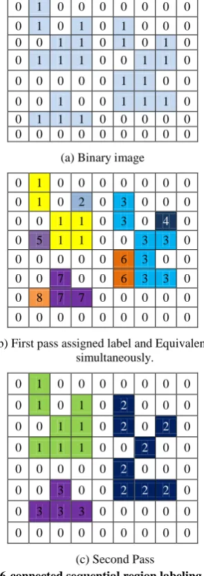
When using the 4-connected neighbourhood N4, only the two neighbours N1 = b(x−1, y) and N2 = b(x, y−1) need to be considered. In proposed algorithm N1, N2 and b(x, y) is upper, left and current pixels value respectively as shown in figure 1.

[image:2.595.311.541.77.588.2]

b(x-1, y) b(x, y-1) b(x, y)

Figure 1: The neighbourhood of pixel b(x, y) in 4-connected connectivity

First Pass:

Each object pixel is assigned a label according to the following criteria:

 First finding the object pixel or foreground pixel b(x, y) it is also known as current object pixel as shown in figure 2(a).

 Finding the upper neighbor b(x-1, y) and left neighbor b(x, y-1) of the object pixel b(x, y).

 If the upper neighbor and left neighbor of the object pixel are background pixels, then increment the new label L (which is initialized to 1) and assigned to the object pixel.

 If the upper neighbor has label X and left neighbor of the object pixel has a different label Y (i.e. X ≠ Y), then assigned minimum neighborhood of both pixel value to the object pixel. These minimum neighborhood pixel values is a provisional label are also assigned in a one dimensional equivalent array. The equivalent table is updated simultaneously as shown in figure 2(b).

 If both the upper neighbor and left neighbor of the object pixel have the same label X, then assigned label X to the object pixel.

 If either the upper neighbor or the left neighbor of the object pixel has the label X, then assigned label X to the object pixel. This label is also assigned into the equivalent array. Table 1 shows as provisional label obtained from first pass scanning process.

Table 1: One dimensional equivalent array

Index

Term 0 1 2 3 4 5 6 7 8 9 10

Provisi-onal label 0 1 2 3 2 5 2 5 5 9 9

Object Counting:

 First initialize number of object (say no_obj = 0) by zero.

 If the equivalent array value is equal to say integer I then increase the no_object and replaced equivalent label with new label (representative label) is called representative table otherwise no changed in equivalent array value. This representative array is used in second scanning process. Table 2 shows as representative label.

Table 2: One dimensional representative array

Index term 0 1 2 3 4 5 6 7 8 9 10

Represent-ative label 0 1 2 3 2 4 2 4 4 5 5

 Maximum number of object depending on the representative label set.

0 1 0 0 0 0 0 0 0 0 1 0 1 0 1 0 0 0 0 0 1 1 0 1 0 1 0 0 1 1 1 0 0 1 1 0 0 0 0 0 0 1 1 0 0 0 0 1 0 0 1 1 1 0 0 1 1 1 0 0 0 0 0 0 0 0 0 0 0 0 0 0

(a) Binary image

0 1 0 0 0 0 0 0 0 0 1 0 2 0 3 0 0 0 0 0 4 2 0 3 0 5 0 0 6 4 2 0 0 7 5 0 0 0 0 0 0 8 7 0 0 0 0 9 0 0 8 7 7 0 0 10 9 9 0 0 0 0 0 0 0 0 0 0 0 0 0 0

(b) First pass assigned label and Equivalent table simultaneously.

0 1 0 0 0 0 0 0 0 0 1 0 2 0 3 0 0 0 0 0 2 2 0 3 0 4 0 0 2 2 2 0 0 4 0 0 0 0 0 0 0 4 0 0 0 0 0 5 0 0 4 4 4 0 0 5 5 5 0 0 0 0 0 0 0 0 0 0 0 0 0 0

(c) Second Pass

Figure 2: 4-connected sequential region labeling algorithm (a) Binary image in which the foreground pixel are marked 1 and background pixels are marked 0. (b) After first scan assigning provisional label and equivalent array

simultaneously. (c) After second scan replacing provisional label by representative label.

Second Pass:

[image:2.595.96.241.235.271.2]

(3)

3.2 6-Connected Component Algorithm

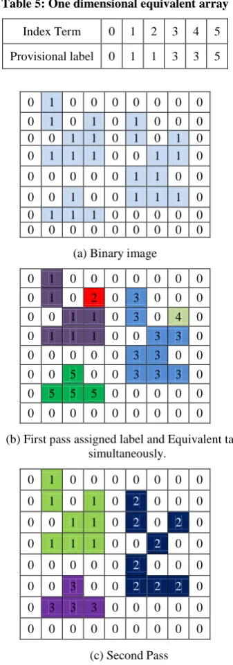
In this algorithm we have used 6-connected neighbourhood N6. For a 2D image, a forward scan assigns labels to pixels from left to right and top to bottom. Each time a pixel is scanned, its neighbors in the scan mask are examined to determine an appropriate label for the current object pixel. In forward scan, all three neighbours N1 = b(x, y-1), N2 = b(x-1, y-1) and N3 = b(x-1, y) must be examined. In the illustration shown in figure 3, the current object pixel being examined is marked as b(x, y).

[image:3.595.354.502.75.492.2]

b(x-1, y-1) b(x-1, y) b(x, y-1) b(x, y)

Figure 3: The neighbourhood of pixel b(x, y) for 6-connected connectivity

First Pass:

 First finding the object pixel or foreground pixel b(x, y) by scanning process. It is also known as current object pixel as in figure 4(a).

 Finding the upper b(x-1, y), left b(x, y-1) and upper-left neighbor b(x-1, y-1) of the object pixel b(x, y).

No Operation

if PO = 0,

b(x, y) = L (L = L + 1) if Po ≠ 0 (Min = 0 & Max = 0),

Emin(x, y) otherwise,

Where:

Min= min[{b(x-i, y-j) | i, j Є Ms}]; Max= max[{b(x-i, y-j) | i, j Є Ms}];

Emin(x, y)= Non-Zero Minimum value; L (which is initialized

to 1) = L+1 indicates an increment of L; PB and PO is the

background and foreground or object pixel in an image respectively; MS is the region of the mask except the object

pixel, i.e. b(x, y-1), b(x-1, y-1) and b(x-1, y); min(.) and max(.) is the operator of calculating minimum and maximum value of the neighboring pixels in the mask, respectively.

 If the object pixel b(x, y) is background pixel there is no change in provisional label.

 If the object pixel belongs to the actual object and both the minimum and maximum values are zero, then increase the provisional label and assigned to the object pixel b(x, y).

 If the minimum value has X and maximum value of the object pixel has a different label Y (i.e. X ≠ Y), then the assign the minimum value (i.e. X) to the object pixel. This minimum value is also assigned in equivalent array is known as provisional label. The equivalent array is updated simultaneously. Figure 4(b) shows that provisional label obtained from first pass process.

Index Term 0 1 2 3 4 5 6 7 8

Provisional label 0 1 1 3 3 1 3 7 7

 If either minimum or maximum value obtained from image has the label X, then assign the label X to the object pixel. This label is also assigned to the equivalent array. Table 3 shows that as provisional label in each index term.

The equivalence array contains a set of provisional label.

0 1 0 0 0 0 0 0 0 0 1 0 1 0 1 0 0 0 0 0 1 1 0 1 0 1 0 0 1 1 1 0 0 1 1 0 0 0 0 0 0 1 1 0 0 0 0 1 0 0 1 1 1 0 0 1 1 1 0 0 0 0 0 0 0 0 0 0 0 0 0 0

(a) Binary image

0 1 0 0 0 0 0 0 0 0 1 0 2 0 3 0 0 0 0 0 1 1 0 3 0 4 0 0 5 1 1 0 0 3 3 0 0 0 0 0 0 6 3 0 0 0 0 7 0 0 6 3 3 0 0 8 7 7 0 0 0 0 0 0 0 0 0 0 0 0 0 0

0 1 0 0 0 0 0 0 0 0 1 0 1 0 2 0 0 0 0 0 1 1 0 2 0 2 0 0 1 1 1 0 0 2 0 0 0 0 0 0 0 2 0 0 0 0 0 3 0 0 2 2 2 0 0 3 3 3 0 0 0 0 0 0 0 0 0 0 0 0 0 0

(c) Second Pass

Figure 4: 6-connected sequential region labeling algorithm (a) Binary image in which the foreground pixel are marked 1 and background pixels are marked 0. (b) After first scan assigned provisional label and equivalent array

simultaneously. (c) After second scan replacing provisional label by representative label.

Object Counting:

 If the equivalent array value is equal to say integer I then increase the no_obj and replaced equivalent label with new label (representative label) is called representative table otherwise no changed in equivalent array value. Table 4 shows representative label in each index term obtained from equivalent table set.

Index term 0 1 2 3 4 5 6 7 8

Representative label 0 1 1 2 2 1 2 3 3

Second Pass:

[image:3.595.86.254.184.220.2]

(4)

create unique labels for each connected component in the image. If representative label and object label are same then no change in label in the image. If both are different labels then assign new label to the object pixel from representative label set. As a result, each connected component is assigned a unique label as shown in figure 4(c).

3.3 8-Connected Component Algorithm

In this algorithm, we have used 8-connected neighbourhood N8. For a 2D image, a forward scan assigned labels to pixels from left to right and top to bottom. Each time a pixel is scanned, its neighbors in the scan mask are examined to determine an appropriate label for the current object pixel. In forward scan, all four neighbours N1 = b(x, y-1), N2 = b(x-1, y-1), N3 = b(x-1, y) and N4 = b(x-1, y+1) must be examined. In the illustration shown in figure 5, the current object pixel being examined is marked as b(x, y).

[image:4.595.345.514.75.556.2]

b(x-1, y-1) b(x-1, y) b(x-1, y+1) b(x, y-1) b(x, y)

Figure 5: The neighbourhood of pixel b(x, y) for 8-connected connectivity

First Pass:

 First finding the object pixel or foreground pixel b(x, y) it is also known as current object pixel as shown in figure 6(a).

 Finding the upper b(x-1, y), left b(x, y-1) upper-left b(x-1, y-1) and upper-right b(x-1, y+1) neighbor of the object pixel b(x, y).

No Operation

if PO = 0,

b(x, y) = L (L = L + 1) if Po ≠ 0 (Min = 0 & Max = 0),

Emin(x, y) otherwise,

Where:

Min= min[{b(x-i, y-j) | i, j Є Ms}] Max= max[{b(x-i, y-j) | i, j Є Ms}]

Emin(x, y)= Non-Zero Minimum value; L (which is initialized

to 1) = L+1 indicates an increment of L; PB and PO is the

background and foreground or object pixel in an image; MS is

the region of the mask except the object pixel, i.e. b(x, y-1), b(x-1, y-1), b(x-1, y) and b(x+1, y-1); and min(.) and max(.) is the operator of calculating minimum and maximum value of the neighboring pixels in the mask respectively.

 If the object pixel b(x, y) is background pixel, then there is no change in provisional label.

 If the object pixel belongs to the same object and both the minimum and maximum values are zero, then increase the provisional label and assigned to the object pixel b(x, y).

 If the minimum value has X and maximum value of the object pixel has a different label Y (i.e. X ≠ Y), then assign minimum value (i.e. X) to the object pixel. This minimum value is also assigned in equivalent array is known as provisional label. The equivalent array is updated simultaneously as shown in figure 6(b).

 If either minimum or maximum value obtained from image has the label X, then assign label X to the object pixel. This label is also assigned into the equivalent array. Table 5 shows provisional label in each index term of one dimensional equivalent array.

The equivalence table contains a set of provisional labels.

Index Term 0 1 2 3 4 5

Provisional label 0 1 1 3 3 5

0 1 0 0 0 0 0 0 0 0 1 0 1 0 1 0 0 0 0 0 1 1 0 1 0 1 0 0 1 1 1 0 0 1 1 0 0 0 0 0 0 1 1 0 0 0 0 1 0 0 1 1 1 0 0 1 1 1 0 0 0 0 0 0 0 0 0 0 0 0 0 0

(a) Binary image

0 1 0 0 0 0 0 0 0 0 1 0 2 0 3 0 0 0 0 0 1 1 0 3 0 4 0 0 1 1 1 0 0 3 3 0 0 0 0 0 0 3 3 0 0 0 0 5 0 0 3 3 3 0 0 5 5 5 0 0 0 0 0 0 0 0 0 0 0 0 0 0

0 1 0 0 0 0 0 0 0 0 1 0 1 0 2 0 0 0 0 0 1 1 0 2 0 2 0 0 1 1 1 0 0 2 0 0 0 0 0 0 0 2 0 0 0 0 0 3 0 0 2 2 2 0 0 3 3 3 0 0 0 0 0 0 0 0 0 0 0 0 0 0

(c) Second Pass

Figure 6: 8-connected sequential region labeling algorithm (a) Binary image in which the foreground pixel are marked 1 and background pixels are marked 0. (b) After first scan assigned provisional label and equivalent array

simultaneously. (c) After second scan replacing provisional label by representative label. Object Counting:

Index term 0 1 2 3 4 5

Representative label 0 1 1 2 2 3

[image:4.595.81.255.255.284.2]

(5)

shows representative label in each index term obtained from equivalent table.

Second Pass:

Again the image is scanned pixel by pixel from left to right and top to bottom. The representative label set is merged to create unique labels for each connected component in the image. If representative label and object label are same then no change in label in the image. But both are different label then assign new label to the object pixel from representative label set. As a result, each connected component is assigned a unique label as shown in figure 6(c).

3.4 Median Filter Algorithm

In median filtering, the input pixel is replaced by the median of the pixels contained in its neighbourhood. There are two main step of proposed algorithm:

Step 1: Choice of the window size

First choose the window size of the median filter. Generally, the size of the neighborhood is chosen as odd number so that a well defined center values exits. In proposed algorithm considers 3X3 window size of the filter.

[image:5.595.314.538.70.338.2]

w(x-1, y-1) w(x-1, y) w(x-1, y+1) w(x, y-1) w(x, y) w(x, y+1) w(x+1,y-1) w(x+1, y) w(x+1, y+1)

Figure 7: Window size 3x3

Let W denote window size of median filter (i.e. 3x3) and for a pixel w(x,y) denoted as central pixel. Window size is increasing to remove better noise but it will take time. A sliding window size is calculated by (2L + 1)  (2L + 1) where L denoted in any integer. The elements of this window are Sx, y = {Wx-i, y-j, -L≤ i, j ≤ L} as shown in figure 7.

Step 2: Filtering Operation

Sliding the window on image from top to bottom and left to right. Window W is suitably chosen neighborhood pixels value. The algorithm for median filtering requires arranging the pixel values in the neighborhood in ascending or descending order and picking up the value at the center of the array. If, however, the size of the neighborhood is even then the median is taken as the arithmetic mean of the two values at the center.

4. EXPERIMENT RESULTS

4.1 Object Counting Results

The goal of this experiment is to measure the performance of three algorithms (4-connected, 6-connected and 8-connected) on binary images (obtained by thresholding the gray label image, Pixels with a grey level above the threshold are set to 1 (equivalently 255), whilst the rest are set to 0) are converted from color or grayscale images. In this experiment various types of images are used. The images are regular, irregular, impulse noises images in which the objects are distinct and are not matched to the background. These proposed algorithms can be applied any image format. All of these images in color or grayscale are transformed into binary images by a proper threshold value. Figure 8 shows that different types of images have taken for resulting purpose.

(a) (b)

(c) (d)

(e) (f)

[image:5.595.90.246.327.393.2]

(g) (h)

Figure 8: Tested images with different background, left side (a, c, e, g) are input images and right side (b, d, f, h)

are converted binary images

4.2 Median Filter Result

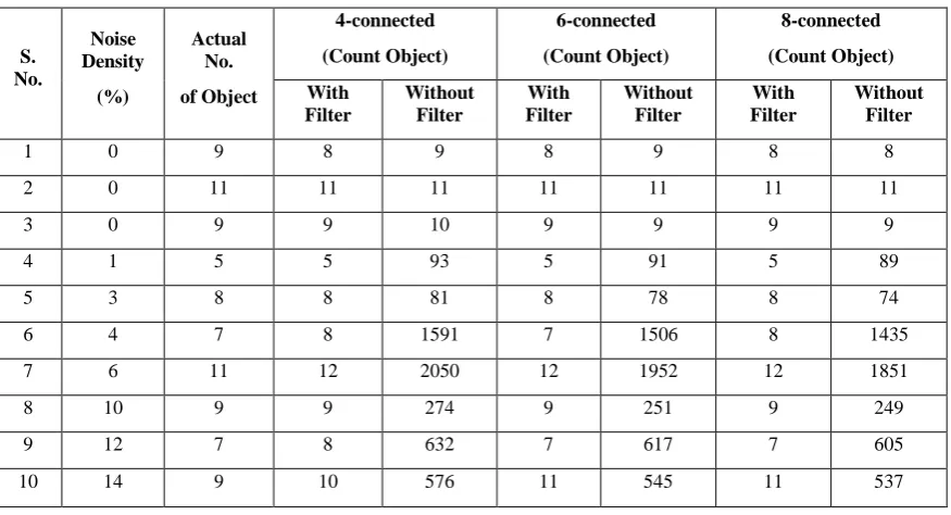
The Proposed Algorithm is tested using gray scale, color and binary images of different size and file format. Some images can be corrupted by salt & pepper noise with equal probability. Proposed algorithm is found to perform quite well on image corrupted with salt & pepper noise. Experimental result only shows the noise density variations from 1% to 20%. The Figure 9 shows one image having equal noise density of 6% after passing through different window size.

(a) Original Image (b) Noise Ratio 6%

(c) Window size 3x3 (d) Window sizes 5x5

(e) Window sizes 7x7

[image:5.595.314.537.483.737.2]

(6)

Table 7: Counting Object by using proposed algorithm in binary images

S. No.

Noise Density

(%)

Actual No.

of Object

4-connected

(Count Object)

6-connected

(Count Object)

8-connected

(Count Object)

With Filter

Without Filter

With Filter

1 0 9 8 9 8 9 8 8

2 0 11 11 11 11 11 11 11

3 0 9 9 10 9 9 9 9

4 1 5 5 93 5 91 5 89

5 3 8 8 81 8 78 8 74

6 4 7 8 1591 7 1506 8 1435

7 6 11 12 2050 12 1952 12 1851

8 10 9 9 274 9 251 9 249

9 12 7 8 632 7 617 7 605

[image:6.595.81.519.85.322.2]

10 14 9 10 576 11 545 11 537

Figure 10: Performance comparison of connected component algorithms on binary images.

5. ACCURACY

Calculated Accuracy through some steps:

Error = (Actual number of object – counted object) //only taken positive value;

Error E (%) = [Error/actual number of object]*100 //Each image calculate error

Average Error (%) = //n = Number of image;

Accuracy (%) = 100 - Average Error (%);

4-Connected Component Algorithm

Calculated Accuracy with filter Average Error (%) = 5.81 Accuracy (%) = 94.19

6. CONCLUSION

This paper has attempted to evaluate the performance of three types of object counting method and one of noise removing method, namely the 4-connected, 6-connected, 8-connected and median filter algorithm. In practically in all cases, the technique had successfully given the desired result on binary image. Experimental result shows that the proposed 6-connected method has provided better result as compare to 8-connected or 4-8-connected method. All techniques, some images which are not corrupted from noise have given better accuracy. But the images which are corrupted from salt and pepper noises have given very poor accuracy but to have given better accuracy after de-noising the image by median filter. So this proposed algorithm of 6-connected with median filter is better than 8-connected and 4-connected methods with median filter.

7. FUTURE SCOPE

In this paper we discussed about 4-connected, 6-connected and 8-connected component labeling algorithm for counting objects from images. We used median filter to remove the salt and pepper noise to give better results. Further enhancements in proposed algorithms are to develop other type of filter for de-noising the different type of noise and can be further improved by using improved connected component labeling algorithm. These methods will be helpful for object based analysis and object finding algorithm.

8. REFERENCES

[1] Akmal Rakhmadi, Nur Zuraifah Syazrah Othman, Abdullah Bade, Mohd Shafry Mohd Rahim and Ismail Mat Amin (2010), “Connected Component Labeling Using Components Neighbors-Scan Labeling Approach” Journal of Computer Science, ISSN 1549-3636, 6 (10): pp 1099-1107.

[2] Mark A. Foltz (1997), Connected Components in Binary Image 6.866: Machine Vision December 15.

(7)

Components in Binary Images” WCE July 4 - 6, 2012 vol II, London, U.K., ISBN: 978-988-19252-1-3. [4] Roshan Dharshana Yapa and Koichi Harada (2008),

“Connected Component Labeling Algorithms for Gray-Scale Images and Evaluation of Performance using Digital Mammograms” International Journal of Computer Science and Network Security, VOL.8 No.6, pp 33-41.

[5] Tinku acharya and Ajoy K. Ray (2005) “Image Processing Principles and Applications”, A John Wiley and Sons Inc., Publication, ISBN-10: 0471719986, pp 152, 311-312.

[6] Gonzalez R.C., and Woods R.E. (2002) “Digital Image Processing” (Second Ed), Prentice Hall, ISBN-10: 0201180758.

[7] Kenji Suzuki, Isao Horiba, and Noboru Sugie (2003), “Linear-time connected-component labeling based on sequential local operations” Computer Vision and Image Understanding, pp 1-23.

[8] K.B. Wang, T.L. Chia, Z. Chen (2003), “Parallel execution of a connected component labeling operation on a linear array architecture”, J. Inf. Sci. Eng. 19, pp. 353–370.

[9] P. How-Lung Eng and Kai-Kuang Ma (2001), “Noise Adaptive Soft-Switching Median Filter” IEEE Transactions On Image Processing, Vol. 10, No. 2. [10]V.R.Vijaykumar, P.T.Vanathi, P.Kanagasabapathy and

D.Ebenezer (2009) “Robust Statistics Based Algorithm to Remove Salt and Pepper Noise in Images” World Academy of Science, Engineering and Technology 35. [11]B Ravi Kiran, K R Ramakrishnan and Y Senthil Kumar,

Anoop K P, “An Improved Connected Component Labeling by Recursive Label Propagation” Using Divide and Conquer Approach.

[12]JM Park, CG Looney, HC Chen (2000), “Fast Connected Component Labeling Algorithm Using A Divide and Conquer Technique”, Conference on computers and their Applications.

[13]Kesheng W., Ekow O., and Arie S. (2005), “Optimizing Connected Component Labeling Algorithms” In Proceedings of SPIE Medical Imaging Conference, pp. 1965-1976.

[14]Hanan Samet and Markku Tamminen (1986) “An Improved Approach to connected component labeling of images”, International Conference on Computer Vision and Pattern Recognition, pp. 312–318.

[15]Hanan Samet (1981) “Connected Component Labeling Using Quadtrees”, Journal of the ACM - Volume 28, Issue 3, pp. 487 – 501.

[16]Liu Qing, Tang Linbo, Zhao Baojun, Sun Jingle (2012), “A Fast Target Tracking Algorithm Basted on Connected Component Labeling and Grey Value Statistics”, International conference, pp 1267-1270.

[17]He, L., Chao, Y., Suzuki, K. (2007), “A Linear-Time Two-Scan Labeling Algorithm”, IEEE International Conference on Image Processing, vol. 5, PP. 241–244. [18]Computer Vision CITS4240 “Binary Images” School of

Computer Science & Software Engineering The University of Western Australia.

[19]Kesheng Wu, Ekow Otoo, Kenji Suzuki, “Optimization Two-Pass Connected Labeling Algorithm” Science of U.S. department of Energy under contract no. DE-AC03-76SF00098.