Solution of 1D Poisson Equation with Neumann Dirichlet and Dirichlet Neumann Boundary Conditions, Using the Finite Difference Method

(1)

http://dx.doi.org/10.4236/jemaa.2014.610031

Solution of 1D Poisson Equation with

Neumann-Dirichlet and Dirichlet-Neumann

Boundary Conditions, Using the Finite

Diﬀerence Method

Serigne Bira Gueye, Kharouna Talla, Cheikh Mbow

Département de Physique, Faculté des Sciences et Techniques, Université Cheikh Anta Diop, Dakar-Fann, Sénégal

Email: [email protected]

Received 19 May 2014; revised 16 June 2014; accepted 11 July 2014

This work is licensed under the Creative Commons Attribution International License (CC BY). http://creativecommons.org/licenses/by/4.0/

Abstract

An innovative, extremely fast and accurate method is presented for Neumann-Dirichlet and Di-richlet-Neumann boundary problems for the Poisson equation, and the diffusion and wave equa-tion in quasi-staequa-tionary regime; using the finite difference method, in one dimensional case. Two novels matrices are determined allowing a direct and exact formulation of the solution of the Poisson equation. Verification is also done considering an interesting potential problem and the

sensibility is determined. This new method has an algorithm complexity of O N

( )

, its truncation

error goes like

( )

2

O h , and it is more precise and faster than the Thomas algorithm.

Keywords

1D Poisson Equation, Finite Difference Method, Neumann-Dirichlet, Dirichlet-Neumann, Boundary Problem, Tridiagonal Matrix Inversion, Thomas Algorithm

1. Introduction

Poisson equation is used to describe, in quantitative manner, electrostatic and magnetostatic phenomena. It also helps to understand diffusion and propagation related problems, in quasi-stationary regime. Its solution is of great interest for a wide range of fields such as engineering, physics, mathematics, biology, chemistry, etc.

(2)

which are dependent on its Right-Hand Side (RHS). A recent study [1], concerning the case of one dimension, has proposed a direct, exact, and closed formulation of the inverse matrix; independently on the RHS. This in-verse matrix has allowed getting a new, extremely fast solution to the Poisson equation. However, this innova-tive solution, obtained with the finite difference method, discussed only the case of boundary conditions of type: Dirichlet-Dirichlet (DD).

In the present study, we focus on the Poisson equation (1D), particularly in the two boundary problems: Neu-mann-Dirichlet (ND) and Dirichlet-Neumann (DN), using the Finite Difference Method (FDM). Essentially, at-tention is given to the matrices extracted from the algebraic equations from this differential method. Furthermore, an exact formulation of their inverses, independently of the RHS, is determined. Therefore, a new and advanced formulation of the solution to the Poisson equation, is found, for Neumann boundary conditions.

The proposed method is more accurate and faster than the Gaussian elimination method and that of Thomas. In addition, it completes the work made by Gueye S. Bira [1], where the Dirichlet-Dirichlet problem was pre-sented and treated very rigorously and clearly. Here, we determine two matrices that constitute, with the one in ref. [1], a set of solutions, which will contribute greatly to the advance of research in the field of numerical solving of differential equations. They will also permit an extremely exact and simple formulation of the solu-tion to the Poisson equasolu-tion.

We will first consider an ND boundary problem and establish the corresponding algebraic equations coming from the application of the finite difference method, using the centered difference approximation (second order derivative). Then, we will, based on these algebraic equations, and considering the boundary conditions; estab-lish the matrix equation. Thereafter, we discuss the properties of the associated matrix and then, determine its inverse, exactly and independently of the RHS. This will allow a direct and exact formulation of the solution to the Poisson equation for a 1D problem with ND boundary conditions. Complexity, accuracy, and stability are discussed and compared with other methods: Gaussian elimination algorithm and Thomas. Moreover, a verifica-tion of this new method is done by considering an interesting potential problem with inhomogeneous ND boun-dary conditions. The results are compared to the exact analytical solution and show great agreement. A similar approach is followed in the case Dirichlet-Neumann problem. The exact formula of the inverse matrix is deter-mined and also the solution of the differential equation.

2. 1D Poisson Equation with Neumann-Dirichlet Boundary Conditions

We consider a scalar potential Φ

( )

x which satisfies the Poisson equation ∆Φ

( )

x = f x

( )

, in the interval

] , [a b , where f is a specified function. Φ

( )

x fulfills the Neumann-Dirichlet boundary conditions

( )

a a

′ ′

Φ = Φ and Φ

( )

b = Φ_b. An appropriate discretization is chosen, as shown in Figure 1.

The mesh is composed of N+1 discrete points belonging to the interval

[ ]

a b, ; and an extra, imaginary

point, x₀, which is not within this range [2] [3]. With the following step size: x

(

b a

)

h N −

∆ = = , the mesh points

( )

xi are defined by the following relation: xi = + − ⋅a

(

i 1

)

h, i=0,1,,N+1. We denote by Φi the ap-

proximate value of the desired potential at point x_i: Φ ≈ Φ_i

( )

x_i . For each point x_i in the interval [ , ]a b , the value of the right-hand side function is: f_i= f x

( )

_i .

( )

i xi

′ ′

Φ = Φ and Φ = Φ_i′′ ′′

( )

x_i are the first and second derivative of the potential function Φ, respectively, at point x_i. With the centered difference approximation

(

O h

( )

2

)

[2] [4], one gets the first derivative:

( )

2

1 1

2

i i

i O h

h

+ −

Φ − Φ ′

Φ = + (1)

and the second derivative:

(3)

( )

2

1 1

2

, 2, 3, , .

i i i

i O h i N

h

− +

Φ − Φ + Φ ′′

Φ = + = _ (2)

Thus, the discretized 1D Poisson equation becomes a set of algebraic equations:

2

1 2 1 , 2, , .

i− i i+ h fi i N

Φ − Φ + Φ = = _ (3)

The boundary x₁=a must be carefully handled with the extra imaginary point x₀. Combining (1) and (3) for i=1, the effect of the imaginary point is eliminated:

2 1

1 2 .

2 a

f

h h ′

−Φ + Φ = + Φ (4)

One sees that this extra point does not affect the result. It is also to remark that the truncation error goes like

( )

(

2

)

O h [2]. Therefore, this additional point helps to still use the centered difference approximation, even at boundary point

a

.

We can introduce the vector F which elements F_i are defined by:

2 1 2 2

1 , , and , 2, 3, , 1.

2 a N N b i i

f

F =h + Φh ′ F =h f − Φ F =h f i=  N− (5)

Thus, one obtains the following matrix equation:

2 1 1 2 2 2 2 3 4 5 1 : :

1 1 0 0 0 0

2

1 2 1 0 0 0

0 1 2 1 0 0

0 0 1 2 1 0

0 0 0 1 2

0

0 0 0 0 1

0 0 0 0 0 0 1 2

a N N f h h h f h f − = = ′ Φ

−   + Φ

 

 

 ₋ _…  _Φ

 

 −  Φ

    Φ − _ _  _× ₌  

 ₋  _Φ

 

  _Φ

 

 ₋   _Φ 

_{}_ ___                      A Φ 3 2 4 2 5 2 1 2 : N N b h f h f h f h f − =                        

 _{− Φ} 

_{} 

F

(6)

The centered difference approximation leads to an N × N-matrix A=

( )

a_ij that is diagonally dominant, tri-diagonal, negative definite, and symmetric.

3. The Inverse of the Matrix

A

The inverse of the matrix A, denoted B=

( )

b_ij , is also symmetric. It has the following properties:

1 1 2

2

1 2 3

1 1

1

2

, 1 , 2

2

j j j

i i i i

j

i j ij i j i

N

iN iN i

b b

b b b

j N

b b b

b b δ δ δ δ − + − − + =  ₋ ₊ ₌

 _{< <}

 − + =   ₋ ₌  (7)

where j i

δ is the Kronecker’s delta. It also holds:

(

)

(

)

11 11 1 , . 1 , ij

b j i j

b

b i i j

 + − ≤



=  _{+ −} _>

 (8)

The behavior of the determinant and the co-factor of the matrix A in ref. [1] give us also the following rela-tions:

( ) ( )

( )

1 1 11 1 1 1

det 1 , , and 1

1 1 N N N NN N N N N

b N b b

− −

⋅ − −

= − = = − = = − =

− −

(4)

Using the relations in (7)-(9), we can determine exactly the inverse of the matrix A that is associated with our approximation in case of ND boundary conditions. Thus, the coefficients of B are determined with:

(

)

(

)

1 , , 1 ,

ij

N j i j

b

N i i j

− − −  ≤

  

= 

− − −  >

  



(10)

Equation (10) is also equivalent to:

( )

(

)

max , 1 1 .

2

ij

i j i j b = −_N−_ i j − __= −N− +_ + − − _

  

  (11)

Equations (10) and (11) contain the same information. We prefer the first because it appears to be simpler than the latter and can be preferred for an eventual implementation in a programming language.

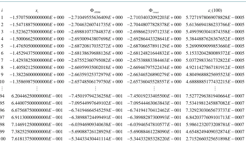
Thus, the inverse matrix is entirely determined. We get the simple, beautiful, exact, and very important matrix B that is shown in Figure 2.

We call this impressive matrix

( )

B , for Neumann-Dirichlet problem: Bira_ND-Matrix. Considering Equa-tion (6), the soluEqua-tion’s vector is obtained with: Φ=BF . Thus, solving the 1D Poisson equation is reduced to a simple matrix-vector multiplication. One does not need an inversion method that depend on the right hand side of the differential equation. Further, the interesting properties of this matrix allow us to get the closed formula-tion of the soluformula-tion, directly without matrix multiplicaformula-tion.

4. Analysis and Exact Solution of the Poisson Equation

The matrix

( )

B is simple and elegant. Only the N first nonzero integers appear in the matrix

( )

B . Its dee-per analysis leads to an exact, closed, and high precise formulation of the solution vector Φ, of the Poisson equation.

With Equation (6), one obtains the solution Φ_N at point x_N with:

1

N

N i

i

F =

Φ = −

∑

(12)

The scalar potential Φ_N₋₁ at abscissa x_N−₁ is given by:

1

2

N

N i N

i

F F

−

=

 

Φ = −_ _− ⋅



∑

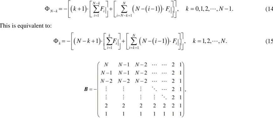
 (13) Thus, the solution of the 1D Poisson equation, in the case of Neumann-Dirichlet boundary, is determined ex-actly with the direct relation:

(

)

(

( )

)

1 1

1 1 , 0,1, 2, , 1.

N k N

N k i i

i i N k

k F N i F k N

−

= = − +

    

Φ = −_ + ⋅_ _{ }+ − − ⋅ __ = −

   



∑

  (14)

This is equivalent to:

(

)

(

( )

)

1 1

1 1 , 1, 2, , .

k N

k i i

i i k

N k F N i F k N

= = +

    

Φ = −_ − + ⋅_ _{ }+ − − ⋅ __ =

   

[image:4.595.98.534.515.705.2]



∑

  (15)

(5)

Equation (15) represents a great improvement for solving the Poisson equation, particularly for Neumann- Dirichlet boundary conditions. The solution is determined properly, exactly, and given in a direct formulation. It can be very easily programmed. One loop will be largely sufficient to compute all the solution of one the most important equation in physics and engineering, in the one-dimensional case. It is a novel and exact formulation of the solution with the finite difference method using the centered difference approximation. The very impor-tant matrix B allowed us to obtain this innovative solution.

The methods that use inversion technics to obtained the matrix B (Gauss Elimination

(

O N

( )

3

)

, Thomas Method

(

O N

( )

)

are ameliorated [5].

The presented new solution is more direct, more exact, more stable; and faster than the Thomas Method for 1D Poisson equation. An important fact is that the determination of B does not depend on the right-hand side of the inhomogeneous Poisson equation. While the other methods use an inversion depending on the RHS of the differential equation. Also, this new solution is very economical with respect to the memory occupation. Then, the solution of the 1D Poisson equation can be got, plotted, and exploited without declaring or using an array in a programming code. That is a great improvement in term of efficient use of memory allocation. Now, we can verify the method, using a potential problem with ND boundary conditions.

5. Verification with a Neumann-Dirichlet Potential Problem

We consider a scalar field Φ

( )

x , which satisfies

( )

2

( )

2

( )

0cos

(

0

)

x

x f x V kx

x ϕ

∂ Φ

∆Φ = = = +

∂ ,

in ] , [a b , where a, b, V₀, k, and ϕ₀ are specified real constants. Φ

( )

x fulfills the Neumann-Dirichlet

boundary conditions: the values d

( )

dx a a

Φ _′

= Φ and Φ

( )

b = Φ_b are given. The exact solution is

( )

0

(

) (

)

0

(

)

(

)

exact a sin 0 2 cos 0 cos 0 b

V V

x ka x b kx kb

k

ϕ

k

ϕ

 _′  _ _

Φ = Φ −_ + _⋅ − − _ + − + _+ Φ

  (16)

We can apply the finite difference method, taking: π

2

a= − , π

4

b= , V₀ =1, π

2

k= , ₀ π

4

ϕ = . We define the

mesh according to Figure 1, with N =100, ∆ = =x h

(

b−a

)

N , x_i = + − ⋅ ∆a

(

i 1

)

x, Φ ≈ Φ_i

( )

x_i , and

( )

cos

(

0

)

i i i

f = f x = kx +ϕ . We consider inhomogeneous Neumann-Dirichlet Boundary conditions: 1

4

a

′ Φ =

and 1

2

b

Φ = − .

Then, we compute the solution, with new method, given by Equation (15) and compare it with the exact po-tential (Equation (16)). Naturally, we also take into account the Equation (5).

We denote by ε_i

( )

100 the relative error at point x_i, for

(

N=100

)

. Φ_i_FDM is the potential value calcu-lated with the new method i.e. Φ_i, at mesh point x_i.

For a given N, the relative error is obtained according the follow relation:

( )

FDM exact exact

= i i

i

N

ε Φ − Φ

Φ (17)

The denote ε

( )

N the average value of the relative error for a given N. It is defined by:

( )

1

1 N i i

N N

N

ε ε

=

∑

(18)

It is calculated for the given parameters and its value is: ε

( )

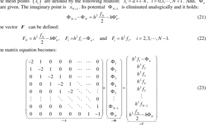
100 ≈1.67681 10× −5. This is a very good accu-racy and corresponds to the results we expected.

(6)

[image:6.595.92.507.99.343.2]

Table 1.Results of the Neumann-Dirichlet problem..

FDM exact (100)

1 1.57075000000000 000 2.71049555636409 000 2.71034032092203 000 5.7271978069078828 0005

2 1.54718875000000 000 2.70463260741735 000 2.70448077828378 000 5.6136694186233766

i i i i

i x

E E E E

ε

Φ Φ

− + − + − + −

− + − + − + −0005

3 1.52362750000000 000 2.69881073784837 000 2.69866231971233 000 5.4993903041874358 0005

4 1.50006625000000 000 2.69300943807698 000 2.69286443328641 000 5.3844887626367652 0005

5 1.4765050000

E E E E

− + − + − + −

− 0000 000 2.68720817035272 000 2.68706657891129 000 5.2690909099853660 0005

6 1.45294375000000 000 2.68138639688126 000 2.68124821644832 000 5.1533204280089372 0005

7 1.42938250000000 000 2.675523

E E E E

E

+ − + − + −

− + − + − + −

− + − 60795082 000 2.67538883384463 000 5.0372983361732822 0005

8 1.40582125000000 000 2.66959935002018 000 2.66946797522434 000 4.9211427867181912 0005

9 1.38226000000000 000 2.66359325372979 000 2.66

E E E

E E E E

E E

+ − + −

− + − + − + −

− + − + − 346526890279 000 4.8049688825695523 0005

10 1.35869875000000 000 2.65748506179750 000 2.65736045528557 000 4.6888885177432215 0005

94 6.20446250000000 001 7.45019794236258 001 7.45019233405500

E E

E E E E

E E

+ −

− + − + − + −

− − − −

    

001 7.5277296381940664 0007

95 6.44007500000000 001 7.09544997649102 001 7.09544463063843 001 7.5341981245887082 0007

96 6.67568750000000 001 6.74194664545259 001 6.74194170412462 001 7.32923030656

E E

E E E E

E E E

− −

− − − − − −

− − − − − 73737 0007

97 6.91130000000000 001 6.38988724499491 001 6.38988287300993 001 6.8420377609101713 0007

98 7.14691250000000 001 6.03946909340638 001 6.03946547810577 001 5.9861232073208781 0007

99 7.382

E

E E E E

−

− − − − − −

52500000000 001 5.69088726128929 001 5.69088461228090 001 4.6548249409032874 0007

100 7.61813750000000 001 5.34433430441114 001 5.34433285328220 001 2.7152660325651898 0007

E E E E

− − − − − −

the centered approximation. It also gives the exact value of the potential

(

Φ_i_exact

)

, obtained by considering the Equation (16) and the relative error at mesh point x_i.

We see that the solution of the ND boundary problem with the proposed method is also very accurate as shown in the table above.

At this stage, we are interested in the sensitivity of this method. We have shown the average relative error

( )

N

ε for different values of N. Then, we got the curve shown in Figure 3, which is a hyperbola. This func-

tion can be assumed to be proportional to

(

)

2

2 2

2 b a

h x

N −

= = ∆ .

A curve fitting of the sensibility can be given with:

( )

2

(

)

2

Trunc N h b a ,

N

α

−

= ⋅ = ⋅ (19)

where α≈3.11729 10× −2. The two curves are shown in Figure 3.

The average relative error ε

( )

N behaves like a truncation error that we express in the following manner ( )4

_{( )}

2 exact

12

hΦ c

. Φ( )_exact4

( )

c is the fourth order derivative of the exact potential function Φ_exact in a point (here

C), which belongs to the interval

[ ]

a b, .

For the given function Φ_exact and also the results from the fitting, we have [6]:

( )

2

(

)

2 2 0 2

2 .

12

b a h V k

N h

N

ε

≈ ⋅

α

= ⋅

α

− < (20)

6. Solution of Dirichlet-Neumann Problem

6.1. Discretization and Matrix Equation

(7)

[image:7.595.144.487.97.365.2]

Figure 3.Sensibility for the Neumann-Dirichlet problem.

Figure 4.Discretization for Dirichlet-Neumann boundary conditions.

Here, the mesh points

( )

x_i are defined by the following relation: x_i = + ⋅a i h, i=0,1,,N+1. And, Φ_a and Φ_b′ are given. The imaginary point is x_N+₁. Its potential ΦN+1 is eliminated analogically and it holds:

2

1 .

2

N

N N b

f

h h

− ′

Φ − Φ = − Φ (21)

Thus, the vector F can be defined:

2 2 2

1 1

, , and , 2, 3, , 1. 2

N

N b a i i

f

F =h − Φh ′ F =h f − Φ F =h f i=  N− (22)

Thus, the matrix equation becomes:

2 1

1 ₂

2

2 ₂

3

3 ₂

4

5

1

: :

2 1 0 0 0 0

1 2 1 0 0 0

0 1 2 1 0 0

0 0 1 2 1 0

0 0 0 1 2

0

0 0 0 0 1

0 0 0 0 0 0 1 1

a

N N

h f h f h f h

−

= =

− Φ Φ

−  

 

 

 ₋  _Φ

 

 −  Φ

 

Φ

− _ _

 _× ₌

 

 ₋  _Φ

 

  _Φ

 

 ₋   _Φ 

_{}_ ___  

        

       

  

A Φ

4 2

5

2 1

2

:

2

N N

b

f h f

h f f

h h

−

′

=

 

 

− Φ

 

_{} 

F

(23)

[image:7.595.126.539.423.674.2]

(8)

6.2. Inverse Matrix and Closed Solution

Thus, the inverse matrix of A can be easily determined from that of the case of ND boundary conditions; using the symmetry in relation to the anti-diagonal. We obtain the beautiful and elegant matrix in Figure 5:

We call this impressive matrix

( )

B , for Dirichlet-Neumann problem: Bira_DN-Matrix. Thus, the exact ex-pression of the solution of the Poisson equation can be formulated in a very simple manner, as following:

1

, 1, 2, , .

k N

k i i

i i k

i F k F k N

−

= =

   

Φ = −__ ⋅ _+ ⋅_ __ =

   



∑

  (24)

This solution, given by the simple and extremely important Equation (24), can be easily computed, in one programming loop that give all the solutions.

7. Verification with a Dirichlet-Neumann Boundary Problem

We consider the same potential as that of the ND boundary problem, studied above. In this DN problem, the

boundary conditions are: d

( )

dx b b

Φ _{= Φ}_′

and Φ

( )

a = Φ_a. The exact solution is obtained by permuting

a

and

b in Equation (16).

We can apply the finite difference method, taking: π

2

a= − , π

4

b= , V₀ =1, π

2

k= , ₀ π

4

ϕ = . We define the

mesh according to Figure 4, with N=100, x h b a N −

∆ = = , x_i = + ⋅ ∆a i x, Φ ≈ Φ_i

( )

x_i , and

( )

cos

(

0

)

i i i

f = f x = kx +ϕ . We consider inhomogeneous DN Boundary conditions: Φ =b′ 1 4 and 1 2

a

Φ = − .

[image:8.595.97.537.470.710.2]

Then, we compute the solution, of our new method, given by Equation (24) and compare it with the exact po-tential.

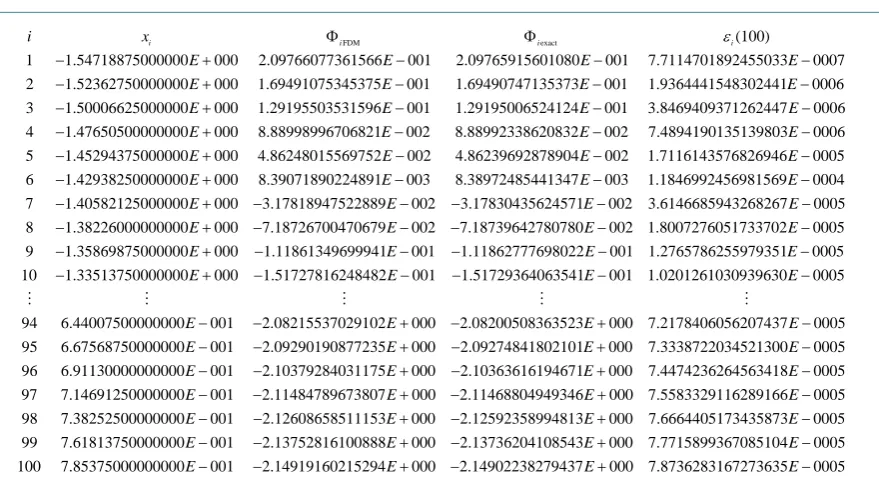
Table 2 shows the obtained results:

The solution of the DN problem is also very accurate as shown in Table 2:

( )

5

100 2.9216432 10

ε _≈ _× −

.

Table 2.Results of the Dirichlet-Neumann problem.

FDM exact (100)

1 1.54718875000000 000 2.09766077361566 001 2.09765915601080 001 7.7114701892455033 0007 2 1.52362750000000 000 1.69491075345375 001 1.69490747135373 001 1.9364441548302441 0006

i i i i

i x

E E E E

ε

Φ Φ

− + − − −

3 1.50006625000000 000 1.29195503531596 001 1.29195006524124 001 3.8469409371262447 0006 4 1.47650500000000 000 8.88998996706821 002 8.88992338620832 002 7.4894190135139803 0006 5 1.45294375000000 00

E E E E

E

− + − − −

− + 0 4.86248015569752 002 4.86239692878904 002 1.7116143576826946 0005 6 1.42938250000000 000 8.39071890224891 003 8.38972485441347 003 1.1846992456981569 0004 7 1.40582125000000 000 3.17818947522889 00

E E E

E E E E

E E

− − −

− + − − −

− + − − 2 3.17830435624571 002 3.6146685943268267 0005

8 1.38226000000000 000 7.18726700470679 002 7.18739642780780 002 1.8007276051733702 0005 9 1.35869875000000 000 1.11861349699941 001 1.11862777698022

E E

E E E E

E E

− − −

− + − − − − −

− + − − − 001 1.2765786255979351 0005

10 1.33513750000000 000 1.51727816248482 001 1.51729364063541 001 1.0201261030939630 0005

94 6.44007500000000 001 2.08215537029102 000 2.08200508363523 000 7.21784

E E

E E E E

E E E

− −

− + − − − − −

− − + − +

    

06056207437 0005 95 6.67568750000000 001 2.09290190877235 000 2.09274841802101 000 7.3338722034521300 0005 96 6.91130000000000 001 2.10379284031175 000 2.10363616194671 000 7.4474236264563418 0005 9

E

E E E E

−

− − + − + −

7 7.14691250000000 001 2.11484789673807 000 2.11468804949346 000 7.5583329116289166 0005 98 7.38252500000000 001 2.12608658511153 000 2.12592358994813 000 7.6664405173435873 0005 99 7.61813750000000

E E E E

E

− − + − + −

001 2.13752816100888 000 2.13736204108543 000 7.7715899367085104 0005 100 7.85375000000000 001 2.14919160215294 000 2.14902238279437 000 7.8736283167273635 0005

E E E

E E E E

− − + − + −

(9)

[image:9.595.242.394.88.176.2]

Figure 5.Inverse matrix for Dirichlet-Neumann problem.

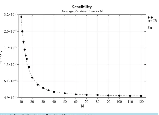
Figure 6.Sensibility for the Dirichlet-Neumann problem.

Now, the sensibility can be determined, for the DN boundary problem: the average relative error ε

( )

N is plotted for different values of N. Then, we got the hyperbola in Figure 6, which can be assumed to be propor-tional to h2.

A curve fitting of the sensibility can be given using Equation (20) with α≈5.504505492 10× −2. The two curves are shown in Figure 6.

The average relative error ε

( )

N goes like O h

( )

2 , which corresponds to the predicted truncation error.

8. Conclusion

This study has determined two novels matrices independently of the RHS providing a new and exact formula-tion of the soluformula-tion of the Neumann boundary problem, for the 1D Poisson equaformula-tion. The presented results and methods constitute a great improvement in the field of solving similar equations: diffusion and wave equations, in the quasi-stationary case, using the FDM. They are direct, highly accurate, extremely fast, and economical in terms of memory occupation.

References

[1] Gueye, S.B. (2014) The Exact Formulation of the Inverse of the Tridiagonal Matrix for Solving the 1D Poisson Equa-tion with the Finite Difference Method. Accepted Manuscript (JEMAA, April 2014).

[2] Engeln-Muellges, G. and Reutter, F. (1991) Formelsammlung zur Numerischen Mathematik mit QuickBasic-Program- men, Dritte Auflage, BI-Wissenchaftsverlag, 472-481.

[image:9.595.149.486.200.444.2]

(10)

[4] LeVeque, R.J. (2007) Finite Difference Method for Ordinary and Partial Differential Equations, Steady State and Time Dependent Problems. SIAM, 15-16. http://dx.doi.org/10.1137/1.9780898717839

[5] Conte, S.D. and de Boor, C. (1981) Elementary Numerical Analysis: An Algorithmic Approach. 3rd Edition, McGraw- Hill, New York, 153-157.