Modified Maximum Likelihood Estimation in Autoregressive Processes with Generalized Exponential Innovations

http://dx.doi.org/10.4236/ojs.2014.48058

Modified Maximum Likelihood Estimation in

Autoregressive Processes with Generalized

Exponential Innovations

Bernardo Lagos-Álvarez1, Guillermo Ferreira1, Emilio Porcu2 1_{Department of Statistics, Universidad de Concepción, Concepción, Chile} 2_{Department of Mathematics, University Federico Santa María, Valpara}

íso, Chile Email: [email protected], [email protected], [email protected]

Received 19 June 2014; revised 8 July 2014; accepted 26 July 2014 Copyright © 2014 by authors and Scientific Research Publishing Inc.

This work is licensed under the Creative Commons Attribution International License (CC BY). http://creativecommons.org/licenses/by/4.0/

Abstract

We consider a time series following a simple linear regression with first-order autoregressive er-rors belonging to the class of heavy-tailed distributions. The proposed model provides a useful generalization of the symmetrical linear regression models with independent error, since the er-ror distribution covers both correlated innovations following a Generalized Exponential distribu-tion. Furthermore, we derive the modified maximum likelihood (MML) estimators as an efficient alternative for estimating model parameters. Finally, we investigate the asymptotic properties of the proposed estimators. Our findings are also illustrated through a simulation study.

Keywords

Autoregressive Time Series Model, Maximum Likelihood, Modified Maximum Likelihood, Least Squares, Generalized Exponential

1. Introduction

The common model for a stationary time series is the stationary and invertible autoregressive model of order

( )

(

)

p AR p where the usual assumption is that the innovations

{ }

_t are identically and independently distri-buted (IID) according to a Gaussian distribution with zero mean and variance 2

0

σ > .

studied the robustness properties of the resulting estimators. In this context, [6] generated non-Gaussian distri-butions through transformations of a Gaussian variate.

[7] considered the Huber M-estimation, which is valid under heavy-tailed symmetric distributions, and uses different forms of contaminated Gaussian to compute the influence functionals (IF) of parameter estimates and gross-error sensitivity for the IF. In this context, [8] and [9] have studied the rate of convergence of the least squares (LS) estimators. It may be noted that M-estimation is not valid for skewed distributions, and has the problem of inefficient estimates for short-tailed symmetric distributions; this has been widely shown by [1] in the classical framework of IID observations.

[10] obtained approximations to some likelihood functions in the context of state space models as considered by [11]. Besides, [12] considered an asymmetric Laplace distribution for the innovations of an autoregressive and moving average model and of a generalized autoregressive conditional heteroscedastic model.

The main proposal of our paper is based on the use of modified likelihood as introduced by [13] [14] and [15]

under the framework of IID observations, in order to estimate the parameters in the context of simple linear re-gression with stationary and invertible autoregressive errors of order one with innovations represented by Gene-ralized Exponential distribution; for more details on these distributions the reader refers to [16]. This method is notorious for giving asymptotically fully efficient estimators (for example, see [17]-[20]).

The outline of the paper is as follows. In Section 2 we define the regression linear model with autoregressive errors, where the underlying distribution of the innovations is a Generalized Exponential distribution. In Section 3 we propose the MML estimators as a powerful methodology to deal with ML estimators which are intractable in the case of a Generalized Exponential distribution. In Section 4 we study the asymptotic properties of the proposed estimators. The main advantages of the proposed estimators are discussed via simulation studies in Section 5. Finally discussions and observations appear in Section 6 of the proposed model and the specific nu-merical results, attaching an Appendix which displays the details of asymptotic results.

2. The Model

We denote

{

Y tt, = ±0, 1,

}

a time series and the following model

1

, .

t t t

t t t

Y µ δX η

η φη

∗ −

= + +

= + (1)

where Xt is the value of a fixed design variable X at time t, ηt is the error, assumed to be modeled through a

non-Gaussian stationary autoregressive model, µ∗ is a constant, φ is the autoregressive coefficient, with

1

φ < , and t is the innovation, distributed according to a Generalized Exponential distribution (GEd), given

by

(

)

(

)

1

; , 1 e t e t, 0, 0, 0.

t t

f  λ α =αλ − −λ α− −λ  ≥ α > λ> (2)

The corresponding cumulative distribution function is given by

(

; ,

)

(

1 e t

)

, 0, 0.

t t

F  λ α = − −λ α  ≥ α> (3)

Notably, λ and α play, respectively, the role of scale and shape parameters. The GEd

(

λ α,

)

has a similar form to the Gamma and Weibull distributions. See the survey in [21] for some recent developments on GEd, distributions.

3. Modified Maximum Likelihood Estimators

The model in Equation (1) can be written as

(

)

{ }

(

)

1 1 , IIDGEd , ,

t t t t t t

Y −φY− = +µ δ X −φX− +   λ α (4)

or

( )

B Y_t

( )

B X_{t t},

φ = +µ δφ + (5)

Conditional on Y0= y0, the likelihood function for the parameter vector

(

µ δ φ α λ, , , ,

)

Τ ₌

β in model (4) is

given by

( )

(

)

1

1

1 e t e t,

n

z z

n n

t

L α λ − α− −

=

=

∏

−

β (6)

where zt=λt, with t =φ

( )

B yt− −µ δφ

( )

B xt or zt =λ

(

wt −µ

)

, wt given by

( )

( )

.

t t t

w =φ B y −δφ B x (7)

The log-likelihood is given by

( )

( )

( )

(

)

(

)

1 1

ln ln 1 ln 1 e t .

n n

z t

t t

l n α λ z α −

= =

= _ + _−

∑

+ −

∑

−

β (8)

For convenience we introduce at this point the following reparameterization: λ: 1= σ and α= −b. Then the density function of t is given by

(

)

(

)

1

e

; , , 0,

1 e

t

t

t b t

b f b σ σ σ σ − + −

= − >

− 



  (9)

where σ >0 and b<0. Its cumulative distribution function is

(

; ,

)

(

1 e t

)

b, 0.

t t

F  bσ = − − σ −  > (10)

Now zt =t σ , and note that

{ }

Zt IID GEd

(

σ =1,b

)

is the standardized member of the GE family. The

log-likelihood for the parameter vector βΤ =

(

µ δ φ σ, , , ,b

)

then becomes

( )

( )

( )

(

)

(

)

1 1

ln ln 1 ln 1 e t .

n n

z t

t t

l n b σ z b −

= =

= _ − + _−

∑

+ +

∑

−

β (11)

Also note that if we consider the parameter b as fixed, then the log-likelihood for the reduced parameter vector, 1

(

µ δ φ σ, , ,

)

Τ₌

β , is proportional to

( )

1

( )

(

)

(

)

1 1

ln 1 ln 1 e t .

n n

z t

t t

l n σ z b −

= =

∝ − −

∑

− +

∑

−

β (12)

For notational simplicity, let us write h z

( )

:=

(

ez−1

)

−1. Then, direct inspection shows that first derivatives of the log-likelihood function with respect to β and β1 can be written as:

( )

( )

₍

₎

_{( )}

( )

( )

₍

_{) (}

_{) (}

_{) ( )}

( )

( )

₍

_{) (}

_{) (}

_{) ( )}

( )

( )

₍

₎

_{( )}

( )

1 1 1 1 1 1 1 1

1 1 1 1

1 1 1 1 1 1 1 , 1 1 , 1 1 , 1 1 , n t t n n

t t t t t

t t

n n

t t t t t

t t

n n

t t t

t t

l l

n b h z

l l

x x b x x h z

l l

y x b y x h z

l l

n z b z h z

l b

µ µ σ

φ φ

δ δ σ

δ δ

φ φ σ

σ σ σ

= − − = = − − − − = = = = ∂ ₌∂ ₌  _{+ +}    ∂ ∂   ∂ ₌∂ ₌  _{− + + −}    ∂ ∂   ∂ ₌∂ ₌  _{− + + −}    ∂ ∂   ∂ ₌∂ ₌ _{− + + +}    ∂ ∂   ∂ ∂

∑

∑

∑

∑

∑

∑

∑

β β β β β β β β

β

_{( )}

1 1 ln . n n t t t t n

z h z

b = =

  = +

∑

+

∑

_{ }

(13)

The likelihood equations are expressions in terms of intractable functions ln e

(

z−1

)

, which lead no explicit solutions, using as alternative numeric iterative methods for get the solutions.

In order to obtain efficient closed form estimators, we consider Tiku’s method of modified likelihood estima-tion, which is by now well established, see [22] (Chapter 6). For given values of µ, δ, b, and φ, let

1:n 2:n n n:

Z ≤Z ≤≤Z be the order statistics of Z1,,Zn. Let µ1:n≤µ2:n≤≤µn n: , with µt n: =

{ }

Zt n: , be the

A standard Taylor expansion of h z

( )

around z=µt n: up to first order allows us to obtain

( )

( )

[

]

( )

:

: : : : : , 1, , ,

t n

t n t n t n t n t t t n

z

h z

h z h z a b z t n

z _µ

µ µ

=

∂

≈ + − = − =

∂  (14)

where

(

:

)

1

:

e t n 1

t t t n

a = µ − − +bµ and _et n:

(

_et n: ₁

)

2

t

b = µ µ − − . A closed form expression for µt n: has been calculated

by [23], namely

(

)

( ) (

)

( )

(

(

)

)

( )

:

0

1 1

1 1 , 1, , ,

1 i n t t n i n t n

b t i t n

i

t n t t i

µ −

=

−

Γ + −  _{  } = _{  }Ψ − + − Ψ _ =

Γ Γ − +

∑

_{+  }  (15)

where ψ

( )

x : d ln= Γ

( )

x dx is the Digamma function. However, for large n, and using the Delta Method, we have the well-known approximation for µt n: for sufficiently large n, µt n: ≈λt n: , with

( )

{

}

(

)

1

1

: : ln 1 ,

1 b

t n t n

t

F F Z

n

λ ₌ − _{= −}  ₋ − 

  ₊  

 

 

 

 (16)

where F−1 is the inverse of the cumulative distribution function of εt, see for instance [22]. Since h z

( )

is

locally linear ([14] [15]), under some very general regularity conditions, zt n: converges to µt n: as the sample

size becomes large, in a small interval not containing the zero value.

Plugging (14) into (13), we obtain the approximated derivative of the log-likelihood function for β1, which

can be written as

( )

1

( )

1

₍

_{) (}

₎

: 1

1

1 ,

n

t t t n t

l l

n b a b z

µ µ σ

∗ = ∂ ∂ ₌  _{+ + −}    ∂  ∂ 

∑

 β β (17)

( )

( )

[ ] [ ]

(

)

(

)

(

_{[ ] [ ]}

)

(

)

1 1 : 1 1 1 1 1 1 , n n

t t t n

t t t t

t t

l l

x φx b x φx a b z

δ δ σ

∗ − − = = ∂ ∂ ₌  _{− + + − −}    ∂  ∂ 

∑

∑

 β β (18)

( )

( )

[ ] [ ]

(

)

(

)

(

_{[ ] [ ]}

)

(

)

1 1 :

1 1 1 1

1 1

1

1 ,

n n

t t t n

t t t t

t t

l l

y δx b y δx a b z

φ φ σ

∗ − − − − = = ∂ ∂ ₌  _{− + + − −}    ∂ ∂ _

∑

∑

_ β β

 (19)

( )

1

( )

1

₍

₎

₍

₎

: : :

1 1

1

1 .

n n

t n t n t t t n

t t

l l

n z b z a b z

σ σ σ

∗ = = ∂ ∂ ₌ _{− + + + −}    ∂ ∂ 

∑

∑

 β β

 (20)

The zeros of the above system of equations are the MML estimators of β1. For the sake of clarity, let

[ ]t y[ ]t δx[ ]t

∆ = − , where y_{[ ]}t and x[ ]t are the concomitants, the associate values of y and x for zt n: , of

[ ]

( )

[ ] : ( )

t n t t

z =_φ B y −δφ B x −µ σ_ . Then, from Equations (17) and (18) we get

( )

_{[ ]}

( )

_{[ ]}

(

( )

_{[ ]}

)

( )

_{[ ]}

( )

_{[ ]}

( )

_{[ ]}

( )

_{[ ]} 1 1 1 1 2

1 1 1 1

1 1 . 1 1 n n n n t t

t t t t

t t

t t

n n n n

t t t t t t t t t

t t t t

b B y a

b b B x

b

b B x b B x b B x B y a B x

b

φ σ

φ _µ

δ

φ φ φ φ σ φ

= = = = = = = =     ₋  ₊       _{   + }    _{  }=     _{ −}  ₊  _   _{ +} _    

∑

∑

∑

∑

∑

∑

∑

∑

Then, from the Equations (17) and (19) we get

[ ] [ ] [ ] [ ] [ ] [ ] [ ] 1 1 1 1 1 2

1 1 1 1

1 1 1 1

1 1 . 1 1 n n n n t t

t t t t

t t

t t

n n n n

t t t t t t t t t

t t t t

b a

b b

b

b b b a

b σ µ φ σ − = = = = − − − − = = = =    _∆  _{∆ −}  ₊       _{   + }    _{  }=   _{∆ ∆}   _{ ∆ ∆ −}  ₊ _{∆ }   _{ +} _    

∑

∑

∑

∑

∑

∑

∑

∑

Defining the n-dimensional vectors, 1=

(

1,,1

)

Τ,

(

b 1

)

11

(

a1, ,an

)

Τ −

= + + _

a , y=

(

y_{[ ]1},,y_{[ ]n}

)

Τ, and

[ ] [ ]

(

x1, ,xn

)

Τ

= 

x , the identities above lead to the following expressions for the MML estimators of β1:

(

)

1

( )

ˆ

ˆ ,

ˆ U DU U D B U

µ

φ σ δ

−

Τ Τ Τ

 

 

= −

  _{ }

 

(

)

1

(

)

ˆ

ˆ _{ˆ ,}

ˆ V DV V D V

µ

δ σ φ

−

Τ Τ Τ

  _{ }

= − −

 

   

  y x a (22)

2 2

4 4

ˆ , or ˆ ,

2 2

c c nd c c nd

n n

σ = + − σ = − − (23)

where



(

1

)



(

( )

)



(

(

)

)

2 2

ˆ ˆ

Diagonal , , n , 1, , 1, ,

n n n n

D b b U φ B V B δ

× =  × = x × = y− x

and

(

)

(

( )

_{[ ]}

( )

_{[ ]}

)

(

)

(

( )

_{[ ]}

( )

_{[ ]}

)

1

2

1

ˆ _ˆ ˆ ˆ

1 1 ,

ˆ _ˆ ˆ ˆ

1 .

n

t t t

t n

t

t t

t

c b a B y B x

d b B y B x b

φ µ δφ

φ µ δφ

=

=

= _ + + _ − −

= + − −

∑

∑

Furthermore, note that setting the expression for ∂l

( )

β ∂b in (13) to zero and solving for b, while substi-tuting zt n: =φˆ

( )

B y_{[ ]}t −δφˆ ˆ

( )

B x_{[ ]}t −µ σˆ ˆ gives

( )

(

[ ] [ ]

)

{

}

(

)

1 1

1

ˆ n _{ln 1 exp ˆ} ˆ ˆ _{ˆ .}

t t

t

b B y x

n µ φ δ σ

− =

 

=

∑

− _ − − _ (24)

We note that the coefficients bt’s are positive. It is expected if the et n: ’s have positive values, then

{ }

(

:

)

ln 1 exp− e_{t n} ’s are all negatives, so ˆb is negative. And if d is negative, no complex roots occur for σˆ.

Moreover 2 2

4

c − nd>c , and _c2_{−4nd >c, resulting as an estimator for} σ_,

(

2

)

ˆ c c 4nd 2n

σ = + − . We observe that these estimates involve the µ parameter.

These facts suggest that it is possible to obtain MML estimators of β by using the following iterative pro-cedure. As a starting point, consider the LS estimator for

(

µ δ φ γ, , ,

)

, with γ = −δφ, which is given by

(

)

1

, , , S L,

µ δ φ γ_    Τ ₌ −

(25)

where

(

1 1 1

)

,

L= ΤY Y X Y Y Y XΤ Τ Τ Τ (26)

(

1, , n

)

,

(

1, , n

)

, 1

(

0, ,1 , n1

)

,

Y = y  y Τ X = x  x Τ X =BX = x x  x₋ Τ (27)

0 1 1

1 1 1

1

1 1 1 1 1 1

1 1 1 1

1 1 1 1 1

1

, and .

1

1 n

y X Y X

y X X X Y X X X

Y BY S

Y Y X Y Y Y X

y X X X Y X X X

Τ Τ Τ Τ

Τ Τ Τ Τ

Τ Τ Τ Τ

Τ Τ Τ Τ

−

 

 

 

 

 

 

=_{ }= _{=  }

 

  _{ }

   

 (28)

We suggest the following routine for the numerical computation of the MML estimator. Initialize with

0 0 0

y = =x and b= −1 (an exponential distribution).

Step 0. Set

(

µ δˆ( )0 ,ˆ( )0,φˆ( )0,γˆ( )0

)

=

(

µ δ( )0 ,( )0 ,φ( )0 ,γ( )0

)

the LSE from (25).

Step 1. Get

(

µ δˆ( )1,ˆ( )1

)

from (21) using

(

φ σˆ( )0, ˆ( )0,b( )0

)

, and φˆ( )1 from (22) using

(

µ δ σˆ( )1,ˆ( )1,ˆ( )0,b( )0

)

. Update σˆ( )1 with (23); b( )1 with (24).

Step 2. Evaluate the expressions (15)-(17) in

(

µ δ φ γ, , ,

)

with the initial estimated values

( ) ( ) ( ) ( )

(

0 _ˆ0 _ˆ0 _ˆ0

)

ˆ , , , .

µ δ φ γ

Step 3. Get from (7) the initial estimates for the w_n =

{

w t_t, =1,,n

}

. Sort the set wn saving the

corres-ponding concomitants values of y yt, t−1, ,x xt t−1, say y[ ] [ ]t,yt−1,x[ ] [ ]t,xt−1.

values vector β( )0.

Step i. Get

(

µ δˆ ,( )i ˆ( )i

)

from (21) using

(

φˆ( )i−1,σˆ( )i−1,b( )i−1

)

, and φˆ( )i from (22) using

(

µ δ σˆ( )i,ˆ( )i,ˆ( ) ( )i−1,bi−1

)

. Update _σˆ( )i

with (23), b( )i with (24).

The steps are repeated until convergence is achieved.

Remark. The stopping criteria is given by

( )

3

1

ˆ ˆ ˆ _{10 .}

s s s

C β = β −β₋ < −

4. Asymptotic Equivalence and Efficiency

The asymptotic equivalence of MML and ML estimators is based on the fact that h z

( )

_{t n:} − −a_t b z_{t t n:} converges to zero as n tends to infinity. Thus, following [17] we have that the differences,

( ) ( )

1n l µ l

( )

1 µ

∗

∂ β ∂ − ∂ β ∂

and

( ) ( )

1n l δ l

( )

1 δ

∗

∂ β ∂ − ∂ β ∂ tend to zero asymptotically. Therefore, the MML and ML estimators are asymptotically equivalent.

On the other hand, if we know the values of φ and σ , asymptotically, the MML estimators µ φ σˆ

(

,

)

and

(

)

ˆ _,

δ φ σ are unbiased for µ and δ . Namely, let 2

(

µ δ,

)

Τ

=

β be the parameter vector and by applying the

standard Taylor expansion in a neighborhood of 2

(

µ δ,

)

Τ

=

  

β we have (see [24])

( )

( )

2 1 2

2 2

2 2 2

2 2

ˆ l l _.

− ∗ ∗ ∂  ∂ = −   ∂ ∂  

 _β

β β

β β

β β

Using the results (5.7.5), p. 115 of [25] and Lemma 1 in the Appendix, we show that 

{

βˆ2−β2

}

=0 for

large n. The unbiasedness property of

(

φ σ,

)

is analogous to the previous case.

Furthermore, if we know the values of φ and σ , the MML estimators µ φ σˆ

(

,

)

and δ φ σˆ

(

,

)

are un-biased and normally distributed with variance-covariance matrix

(

)

2

₍

₎

22 12

2 12 11 22 11 1 1 , . 1 v v v v

n b b v v

σ

φ σ  − 

Σ = _{ }

−

+ − _{ } (29)

knowledge of the values of φ and σ . Observe that

11 12 12 22 1 lim , n v v

U DU b

v v n Τ →∞   = −    

with v11=1, 12 1

( )

[ ]

n

t t

v =

∑

₌φ B x and 22 1

(

( )

_{[ ]}

)

2

n

t t

v =

∑

₌ φ B x . Thus, we have (29) for the asymptotic variance-

covariance matrix of µ φ σˆ

(

,

)

.

The asymptotic behavior of variance for σˆ (say Var

{ }

σˆ ) and φˆ (say Var

{ }

φˆ ) can be deduced from the arguments in [26]. We can thus show that Var

{ }

φˆ 1v33, where

( )1

_{( )}

( )1

₍

_{) (}

)

( )2

₍

₎

33 2

1

1 0; 2 1; 1 1; 2 .

2 b b n

v b b b b

b σ +   = _ − − − + + − + _ +     

Analogously, we have Var

{ }

σˆ 1v₄₄, where

( )

₍

₎

( )

₍

₎

( )

₍

₎

( ) ( )

(

)

(

)

1 1 1

44

1 2 2

1 1; 1 1; 2

1 2

1

2 1; 2 .

2

n b b

v b b b

b b b b b η η η η µ µ σ

µ µ µ σ ∗     = _ + + _{ } − + + − + _ + +       + + + − _{+ } + _   

where ( )j

(

t b k; +

)

is jth derivative of the moment generating function of GEd

(

1,b+k

)

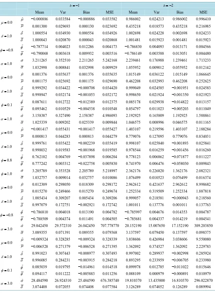
, µη( )r is the rth

[image:7.595.95.538.119.723.2]

Table 1. The simulated values of mean, bias square and mean square error of the LS estimators

(

µ δ φ σ, , ,  

)

and the MML estimators

(

µ δ φ σ, , ,

)

and n=100.

1

b= − b= −2

Mean Var Bias MSE Mean Var Bias MSE

0.0

µ = µ −0.000886 0.033584 −0.000886 0.033582 0.986002 0.024213 0.986002 0.996410

µ 0.001300 0.029693 0.000130 0.023692 0.435218 0.018573 0.435218 0.216985

1.0

δ = δ 1.000554 0.034930 0.000554 0.034926 1.002698 0.024228 0.002698 0.024233

δ 1.000043 0.020870 0.000043 0.020868 1.001481 0.015923 0.001481 0.015923

0.8

φ= − φ −0.787714 0.004023 0.012286 0.004173 −0.786830 0.004093 0.013171 0.004566 φ −0.790068 0.003618 0.009932 0.003516 −0.786149 0.003588 0.013051 0.004480

1.0

σ = σ 3.211265 0.352510 2.211265 5.242168 2.239461 0.176988 1.239461 1.713233

σ 1.032998 0.008841 0.032998 0.009929 1.055952 0.009012 0.055952 0.012142

0.0

µ = µ 0.001376 0.035637 0.001376 0.035635 1.015149 0.036122 1.015149 1.066645

µ 0.001175 0.025692 0.001175 0.029690 0.462208 0.032993 0.462208 0.252625

1.0

δ = δ 0.999292 0.034422 −0.000708 0.034420 0.999049 0.024585 −0.001951 0.024583

δ 0.998947 0.032174 −0.001053 0.032172 0.998650 0.021924 −0.001350 0.021923

0.1

φ = φ 0.087611 0.012722 −0.012389 0.012375 0.085178 0.029938 −0.014822 0.013157 φ 0.095462 0.010529 −0.004538 0.010548 0.054797 0.011023 −0.005203 0.011049

1.0

σ = σ 3.158387 0.327490 2.158387 4.986093 2.192925 0.165809 1.192925 1.588861

σ 1.025339 0.009202 0.025339 0.009844 1.046575 0.008996 0.046575 0.011165

0.0

µ= µ −0.001417 0.055431 −0.001417 0.055427 1.403107 0.219596 1.403107 2.188284

µ 0.000813 0.044283 0.000813 0.044279 0.779076 0.127095 0.779076 0.834031

1.0

δ = δ 0.999761 0.035422 −0.002239 0.035419 0.998107 0.025840 −0.001893 0.025841

δ 0.998032 0.019583 −0.001968 0.019585 0.978544 0.016259 −0.001456 0.016260

0.8

φ = φ 0.762102 0.004769 −0.037898 0.006204 0.778123 0.006862 −0.071877 0.011227 φ 0.777242 0.003312 −0.022758 0.005830 0.741970 0.006476 −0.058030 0.009843

1.0

φ= σ 3.205789 0.353528 2.205789 5.218997 2.362176 0.226820 1.362176 2.082321 σ 1.032757 0.009014 0.032757 0.010086 1.076499 0.010523 0.076499 0.016374

0.0

µ = µ 0.012309 0.298050 0.018309 0.298172 2.962612 0.421637 2.962612 8.998682

µ 0.015270 0.249466 0.015270 0.249674 1.252334 0.319509 1.252334 1.887818

1.0

δ = δ 1.005434 0.309207 0.005434 0.309206 0.999057 0.218581 −0.000943 0.218560

δ 0.997079 0.172751 −0.002921 0.172742 1.001011 0.137776 0.001011 0.137763

0.8

φ= − φ −0.786810 0.004018 0.013190 0.004782 −0.785997 0.004676 0.014353 0.004787 φ −0.788509 0.004374 0.011491 0.004505 −0.785681 0.004337 0.014219 0.004541

3.0

σ = σ 29.042450 29.572310 26.042450 707.778770 20.152190 15.007650 17.152190 309.203850

σ 3.089355 0.071391 0.089355 0.079368 3.137597 0.079450 0.137597 0.098375

0.0

µ = µ −0.009324 0.328285 −0.009324 0.328339 3.038606 0.426984 3.038606 9.550080

µ _−0.006528 0.271379 −0.006528 0.271395 1.362092 0.374527 1.362092 2.229783

1.0

δ = δ 0.991023 0.307443 −0.008977 0.307493 0.997002 0.289937 −0.002998 0.285924

δ 0.996085 0.284231 −0.003915 0.284218 0.893295 0.233959 −0.006705 0.233980

0.1

φ = φ 0.085039 0.019795 −0.014961 0.014518 0.099978 0.012785 −0.011022 0.015646 φ 0.094117 0.011222 −0.005883 0.011256 0.088109 0.000979 −0.000891 0.010979

3.0

σ = σ 28.484590 26.924310 25.484590 676.385740 19.810370 13.435800 16.810370 296.022870

5. Simulation Study

In order to have some indications of the robustness aspects of the MML estimates of µ, δ, φ and σ against LSE estimates, we performed a small numerical study similar to the one presented by [26] for the gene-ralized logistic model. We consider the following AR(1) Genegene-ralized Exponential model:

(

)

{ }

(

)

1 1 , IID GEd ,

t t t t t t

Y −φY₋ = +µ δ X −φX₋ +   λ α (30)

where XtN

( )

0,1 . Additionally, our simulation study considers different scenarios, sketched as follows:

1) µ=0, δ =1, φ= −0.8 and σ =1,

2) µ=0, δ =1, φ=0.1 and σ =1,

3) µ=0, δ =1, φ=0.8 and σ =1,

4) µ=0, δ =1, φ= −0.8 and σ =3,

5) µ=0, δ =1, φ= −0.1 and σ =3.

Without loss of generality, we have considered the parameter b as a constant value given by b = −1 and −2. The summaries of Monte Carlo study for µ, δ , φ and σ , come from the four measures, the mean, 100 × (Bias)2, variance and mean squared error (MSE) for both the LS and the MML estimators. Finally, we use sam-ple size n = 100 and 10,000 replications.Table 1 displays the results from the simulations with the biases, va-riance and MSE of the parameters estimates. The results suggest that the MML estimators are considerably more efficient than the LS estimators for all parameters.

6. Conclusion

In this paper, we have studied a regression linear model with first-order autoregressive errors belonging to a class of asymmetric distributions; more specifically the underlying distribution for the innovations is a Genera-lized Exponential distribution. We have developed a complete asymptotic theory for the MML estimators in these models. In addition, we have shown that the MML estimators are robust and efficient, as depicted by the numerical study presented in Section 5 for the AR(1) GE model. We thus claim that the MML estimator is a very good alternative to estimate autoregressive models with asymmetric innovations (see [26] and [27], among others as example). The R codes may be obtained from the authors upon request in order to analyze such mod-els.

Acknowledgements

The first author would like to thank for the support from DIUC 213.014.022-1.0, established by the Universidad de Concepción. The second author gratefully acknowledges the financial support from ECOS-CONICYT C10E03, established by the Chilean Government and DIUC 213.014.021-1.0 from the Universidad de Concep-ción and the third author was supported by Fodecyt grant 1130647.

References

[1] Tiku, M.L., Tan, W.Y. and Balakrishnan, N. (1986) Robust Inference. Marcel Dekker, Inc., New York.

[2] Tan, W.Y. and Lin, V. (1993) Some Robust Procedures for Estimating Parameters in an Autoregressive Model. Sank-hya B, 55, 415-435.

[3] Damsleth, E. and El-Shaarawi, A.H. (1989) ARMA Models with Double Exponentially Distributed Noise. Journal of the Royal Statistical Society B, 51, 61-69.

[4] Tiku, M.L. (1980) Robustness of MML Estimators Based on Censored Samples and Robust Test Statistics. Journal of Statistical Planning and Inference, 4, 123-143. http://dx.doi.org/10.1016/0378-3758(80)90002-6

[5] Tan, W.Y. (1985) On Tiku’s Robust Procedure—A Bayesian Insight. Journal of Statistical Planning and Inference, 11, 329-340. http://dx.doi.org/10.1016/0378-3758(85)90038-2

[6] Swift, A.L. (1995) Modelling and Forecasting Time Series with a General Non-Normal Distribution. Journal of Fore-casting, 14, 45-66. http://dx.doi.org/10.1002/for.3980140105

[7] Martin, R.D. and Yohai, V.J. (1986) Influence Functionals for Time Series. Annals of Statistics, 14, 781-818.

http://dx.doi.org/10.1214/aos/1176350027

[8] Bhansali, R.J. (1997) Robustness of the Autoregressive Spectral Estimate for Linear Process with Infinite Variance.

[9] Davis, R.A. and Resnick, S. (1986) Limit Theory for the Sample Covariance and Correlation Functions of Moving Av-erages. Annals of the Institute of Statistics, 14, 533-558. http://dx.doi.org/10.1214/aos/1176349937

[10] Durbin, J. and Koopman, S.J. (1997) Monte Carlo Maximum Likelihood Estimation for Non-Gaussian State Space Models. Biometrika, 84, 669-684. http://dx.doi.org/10.1093/biomet/84.3.669

[11] Kitagawa, G. (1987) Non-Gaussian State-Space Modelling of Nonstationary Time Series (with Discussion). Journal of the American Statistical Association, 82, 1032-1063.

[12] Trindade, A.A. and Zhu, Y. (2010) Time Series Models with Asymmetric Laplace Innovations. Journal of Statistical Computation and Simulation, 80, 1317-1333.

[13] Tiku, M.L. (1967) Estimating the Mean and Standard Deviation from Censored Normal Samples. Biometrika, 54, 155- 165. http://dx.doi.org/10.2307/2283834

[14] Tiku, M.L. (1968) Estimating the Parameters of Log-Normal Distribution from Censored Samples. Journal of the Ame- rican Statistical Association, 63, 134-140. http://dx.doi.org/10.2307/2283834

[15] Tiku, M.L. and Suresh, R.P. (1992) A New Method of Estimation for Location and Scale Parameters. Journal of Statis-tical Planning and Inference, 30, 281-292. http://dx.doi.org/10.1111/1467-842X.00072

[16] Gupta, R.D. and Kundu, D. (1999)Generalized Exponential Distributions. Australian and New Zealand Journal of Statistics, 41, 173-188. http://dx.doi.org/10.1111/1467-842X.00072

[17] Vaughan, D.C. and Tiku, M.L. (2000) Estimation and Hypothesis Testing for a Non-Normal Bivariate Distribution with Applications. Journal of Mathematical and Computer Modelling, 32, 53-67.

http://dx.doi.org/10.1016/S0895-7177(00)00119-9

[18] Bhattacharyya, G.K. (1985) The Asymptotics of Maximum Likelihood and Related Estimators Based on Type II Cen-sored Data. Journal of the American Statistical Association, 80, 398-404.

http://dx.doi.org/10.1080/01621459.1985.10478130

[19] Tiku, M.L. (1970) Some Notes on the Relationship between the Distribution of Central and Non-Central F. Biometrika,

57, 175-179. http://dx.doi.org/10.1093/biomet/57.1.175

[20] Tiku, M.L. (1970) Monte Carlo Study of Some Simple Estimators in Censored Normal Samples. Biometrika, 57, 207- 210.

[21] Gupta, R.D. and Kundu, D. (2007) Generalized Exponential Distribution: Existing Methods and Some Recent Devel-opments. Journal of Statistical Planning and Inference, 137, 3537-3547. http://dx.doi.org/10.1016/j.jspi.2007.03.030

[22] Balakrishnan, N. and Cohen, A.C. (1991) Order Statistics and Inference. Academic Press, Waltham.

[23] Raqab, M.Z. and Ahsanullah, M. (2001) Estimation of Location and Scale Parameters of Generalized Exponential Dis-tribution Based on Order Statistics. Journal of Statistical Computation and Simulation, 69, 109-124.

[24] Kendall, M.G. and Stuart, A. (1979) The Advanced Theory of Statistics. Charles Griffin, London.

[25] Tiku, M.L. and Akkaya, A.D. (2004) Robust Estimation and Hypothesis Testing. New Age International (P) Publishers, New Delhi, 337.

[26] Wong, W.K. and Bian, G. (2005) Estimating Parameters in Autoregressive Models with Asymmetric Innovations. Sta-tistics and Probability Letters, 71, 61-70. http://dx.doi.org/10.1016/j.spl.2004.10.022

Appendix

Lemma 1. Let Z GE

( )

1,b , U=exp

( )

−Z , q∈ ∪

{ }

0 and p, s∈ such that p> −b and − < < +1 s b p, then

(

)

{

}

( )

₍

₎

1 p q ;

q s b

E Z U U s b p

b p

− = − + + 

where ( )j

(

t b k; +

)

is jth derivative of the moment generating function of GEd 1,

(

b+k

)

.

Proof

(

)

{

}

₍

_{) (}

₎

₍

₎

( )

₍

₎

1 1

0 0

e e e

1 d e d ; .

1 e 1 e 1 e

q sz z z

p q

q s q sz

Z _z p _z b _z b p

z b b b

E Z U U z z z s b p

b p

− − −

∞ ∞ ₋

+ + +

− − −

− = = = − +

+

− − −

∫

∫



Lemma 2. For the process

{ }

η_t defined as a stationary autoregressive model, ηt =φη εt+ t, φ is the

autoregressive coefficient, with φ <1, and t is distributed according to a GEd. The first and second moment

are given by

( )1 ( )2 2 ( )2

2 and 2 .

1 1

η ε η ε

φ φ

µ µ µ µ

φ φ

= =

− −

Proof is deduced by using the moment generating function of εGEd

(

σ,b

)

(

; ,

)

(

1

₍

) (

1

₎

)

, 1, 1

b t

t b b t

b t

σ

σ σ

σ

Γ + Γ −

= − < <

Γ − +

 (31)

(see [21]). Moreover, for the µη( )1, we used

{ }

{ }

( )1

0

lim lim

k

k k

t t k

k k

j

E η φ E η− φ µ_ε µ_η

→∞ = →∞ +

∑

₌ =

and for µη( )2 , we used

{ }

2 2 ( )2 ( )2 =0

lim lim .

k k t

k k

j

E µ φ µ_ε µ_η