Detection of Malicious Sensor Node in Ad Hoc Sensor
Networks based on Processor Utilization
Deepak Sharma
Shri Mata Vaishno Devi University, Katra, Jammu and Kashmir (INDIA)
ABSTRACT
This paper proposes a strategy based on processor utilization value provided by each sensor node of the network for detecting their malicious activities by comparing the node’s present processor utilization value with the old estimated value .If the difference between the two values is higher or less than the expected value then that particular node become suspicious. A knowledge based system can take decision to expel the malicious node from the network topology
Keywords
Malicious node, Node profile, Threshold value, Regression analysis, Technical efficiency, etc.
1.
INTRODUCTION
A sensor is a device that communicates a physical change in the environment. With the major technological revolutions like connection of sensors to computer systems, the emergence of small, inexpensive and highly reliable micro electronic, and mechanical systems (MEMS) [29] have fuelled the extensive use of sensors. The noble idea of using the dynamic topology of wireless ad-hoc networks and the integration of inexpensive and power efficient reliable sensors in nodes of wireless ad-hoc networks are the driving force behind the great deal of commercial and research interest. There are many cases that determine whether a sensor is malfunctioning for examples there can be a situation when a sensor is reporting erroneous data due to exhausting its energy supply . Energy consumption is one of the most important metrics for wireless ad hoc sensor networks because it directly relates to the operational lifetime of the network ,The sensor’s lifespan is proportional to its power supply. Sensor consumes its energy while transmitting and receiving bits of information. The average amount of energy needed to send or receive information is a bit of data about 4000 nanojoules but the computing and processing data also need extra energy by the sensor. Wireless sensor networks is a special class of ad-hoc networks which efficiently use high node density with keen attention to energy consumption because it has to operate for about five to ten years in terrain conditions .The ability to detect its malfunctioning is critical to the security of any sensor network .The ability to detect a malicious wireless sensor is very difficult because the possibilities for abnormality are endless and moreover, the wireless medium's performance is difficult to predict and control. The wireless channels performance include low bandwidth, high delay, high bit error rates, power and distance tradeoffs, and high packet drop rates .Another malfunction can occur when
a sensor is hacked by an unauthorized person or it is physically damaged by someone. There might be a situation when sensor reporting erroneous data because of hardware or software
problem. The code can be rewritten and would be able to read depending upon the sensor architecture .If the reading and rewriting of the software is not needed for application, then security for that network could be set very high using tamper proof hardware, leaving no chance for the node usage for malicious purposes in case of capturing by an attacker. Keeping the cost effective criterion in mind most of the time, nodes are used on which read /rewrite of the codes can be formed. If an important application installed on the node is hacked by a hacker then changed are made in the application for malicious purpose i.e. with wicked or mischievous intentions or motive and deployed again in place in a mobile Ad hoc network. Now we are having a malicious node having the same hardware ,same id ,also having the same features of the original authenticate node but having altered application for mischievous intentions or motives, and this may leads to corruption of network. To avoid the corruption of the network through captured node or duplicate node, immediate detection of the malicious nodes should be done and then immediately it must be expelled from the Ad hoc network.
2. RELATED WORK
During the past few decades, there has been an fast development growth in the various types of products and services based on utilizing information by monitoring and measuring different types of sensors. A sensor’s node monitors and quantifies parameters which are under investigation. A sensor node responds to an input quantity by generating a functionally related output usually in the form of an electrical or optical signal. Sensing principles include mechanical, chemical, thermal, electrical, chromatographic, magnetic, biological, fluidic, optical, ultrasonic and mass sensing.
Habitat Monitoring constructs a network that consists of many nodes on a monitored landscape and streaming useful live data. Chemical Vapour Sensor System, uses Artificial Neural Networks (ANN) in a wide variety of data processing applications where real-time data analysis and information extraction is required .Optical Sensor System employs an array of optical sensors and identifies the composition of chemical dyes in solution by making use of ANN and optical sensors. High-Energy Shaker Monitoring networks use equipment that generates displacements and accelerations that are capable of shaking sand from huge castings and feeding railroad-car size loads of coal and lumber across conveyors at a specific rate .All these above network applications are programmed to monitor events on land, in the sea, in the air, in plants and in animals depending upon the requirement or the type of networks. The actual network employed depends on the type of applications needed to monitor the physical quantity being measured and are categorized into three types:
1. Node to base station communication, 2. Base station to node communication.
3 Base station to all nodes or reprogramming of the applications on the nodes.
Sensor networks are comprised of thousands of nodes, where each node is a sensor, i.e. pronounced as sensor nodes. Each sensor nodes co-operate to carry out some task assigned to it .These are used to guide itself and others nodes as well as to control data collection and aggregation. The main security goal of each node in the network is to address communication patterns followed by each specific networks. Generally, the sensor networks may be deployed in non-trusted locations. The integrity of the each sensor node can be realized through dedicated secure communications .From the security point of view, wireless communication is fundamentally untrustworthy because of its data broadcast nature .Any adversary can eavesdrop on the traffic, and inject new messages or replay and change old messages. As these sensors node are exposed to hostile environments, the security of sensors is categorized into four main requirements:
1. Data Confidentiality, concerned with data leaking from a sensor to an unintended
recipient.
2. Data Authentication, allows the recipient to verify that the data did indeed come from the claimed sender.
3. Data Integrity, ensures the receiver that the data was not tampered with on its route
4. Data Freshness , means that the data is recently sent.
The security method varies with the type of network i.e. not one size fits all. Various security measure are deployed to protect all the networks. Techniques like traffic encryption key, key cryptography, threshold cryptography, certificate repository, watchdog and pathrater, and reverse metempsychosis.Some other various types of malicious attack performed by the captured node and their intension is to disrupt the network .To avoid the disruption caused by malicious node various techniques have been proposed for the detection of malicious node in the Ad Hoc network.Based on the reputation-based scheme ,a node may drops some or all packets forwarded to him .This was solved by Reputation -based Scheme which uses both self-observation and second hand information to establish compressive reputation of a node. Node with bad compressive reputation will be excluded from the network. The local reputation is not only related to the node’s packet-forwarding ratio (the proportion of correct forwarded packets with respect to the total number of packets to be forwarded during a fixed time), but also related to the busy state of the nodes. The reputation is calculated by R(a,b)=(1-α)* Rold(a ,b) + α* Rcur(a ,b),where Rold = Old reputation and Rcur = New reputation [1]. Another
mitigate the effect of a flooding attack in the AODV protocol. This technique is based on statistical analysis to detect malicious RREQ floods and avoid the forwarding of such packets. As proposed P. Yi et al, in this approach, each node monitors the RREQ it receives and maintains a count of RREQs received from each sender during the preset time period. The RREQs from a sender whose RREQ rate is above the threshold will be dropped without forwarding. Unlike the method proposed in [4], where the threshold is set to be fixed, this approach determines the threshold based on a statistical analysis of RREQs. The key advantage of this approach is that it can reduce the impact of the attack for varying flooding rates.
In a link spoofing attack, a malicious node advertises fake links with non-neighbours to disrupt routing operations. A location information-based detection method was also proposed [5] to detect link spoofing attack by using cryptography with a GPS and a time stamp. This approach requires each node to advertise its position obtained by the GPS and the time stamp to enable each node to obtain the location information of the other nodes. This approach detects the link spoofing by calculating the distance between two nodes that claim to be neighbors and checking the likelihood that the link is based on a maximum transmission range. The main drawback of this approach is that it might not in a situation where all MANET nodes are not equipped with a GPS. Furthermore, attackers can still advertise false information and make it hard for other nodes to detect the attack. In [6], the authors show that a malicious node that advertises fake links with a target’s two-hop neighbors can successfully make the target choose it as the only MPR. Through simulations, the authors show that link spoofing can have a devastating impact on the target node. Then, the authors present a technique to detect the link spoofing attack by adding two-hop information to a HELLO message. In particular, the proposed solution requires each node to advertise its two-hop neighbors to enable each node to learn complete topology up to three hops and detect the inconsistency when the link spoofing attack is launched. The main advantage of this approach is that it can detect the link spoofing attack without using special hardware such as a GPS or requiring time synchronization. One limitation of this approach is that it might not detect link spoofing with nodes further away than three hops. Daniel-Ioan Curiac,Ovidiu Banias,Octavian Dranga proposed a for the detection of malicious node if the application on the captured node is altered, this strategy based on the past and present values provided by each sensor of a network for detecting their malicious activity. Basically, every moment it compare sensor’s output with estimated value computed by an auto regression predictor. If the difference between the two values is higher than a chosen threshold, the sensor node becomes suspicious and a decision block is activated. These solutions can also a way to discover the malfunctioning nodes.
The prediction value can be obtained from the following equation
yA(t)=node1(t) . node1 (t-1) + node2 (t). node2 (t-1) +………+node n(t) . node n(t-1)
(error) eA(t)=xA(t)- yA(t). {Comparing with the present (xA(t)) and estimated value (yA(t))} .If the error is greater than the threshold, then sensor node becomes suspicious and a decision block is activated-[7].
3.
PROPOSED MODEL
Statistical modelling is among the earliest methods used for detecting malicious activity in electronic information systems. It is assumed that an intruder’s behavior is noticeably different from that of a normal behavior, and this model is used to aggregate the sensor node’s behavior which distinguishes an attacker from a normal node behavior. Our statistical techniques
is applicable to program or application running on any node. The observed behavior of a sensor node is flagged as a potential malicious if it deviates significantly from the sensor node’s expected behavior or from different nodes in the same Ad hoc network. The expected behavior of a node is stored in the profile of the server node of the Ad hoc network. Processor utilization mean measures are used to measure for detecting malicious activity of the node.
This algorithm analyzes a node’s activities according to a four-step process.
First, the algorithm generates different data collected vectors to represent the activities of a particular node by monitoring the processor utilization for some time period after some interval of time. Let the different collected vectors generated represented by X1, X2 at different time T = <t1, t2, …, tn>.The session vector Xi =<x1, x2, …, xn > represents the data’s collected from a single session.
Second, A threshold value range is calculated from different X1,X2……where X1 = <x11, x12, …, xmn >, X2 = <x21, x22, …, xpn >, XN , at different interval of time T 1= <t1, t2, …, tn>, T 2= <t1, t2, …, tn>, ………. Tn where <ti is min, ti is max. > by calculating means of acquired different set of data vectors at different interval of time T 1= <t1, t2, …, tn>, T 2= <t1, t2, …, tn> . The threshold value range is formed from different X1,X2…… . The threshold value range is then stored for a particular’s node profile at the server of the network. Let the generated threshold value for a particular sensor node is represented by Vn. Same process is repeated for each node in the network and for each node a threshold value range is made and then stored for a particular’s node profile at the server of the network, only if nodes differ in their application or architecture /manufacture.
Third, this step in the algorithm to detect the malicious activity of particular node. A session vector is formed which represent the activities of a particular node for the current a session by monitoring the processor utilization is acquired for a time period with some fixed interval T 1= <t1, t2, …, tn>, .The time interval and the size of the vector should be same as adjusted during the formation of the threshold range. The already calculated threshold value formed by acquiring different set of data vectors at different interval of time T = <t1, t2, …, tn>, where <ti, min, ti, max> is compared with the current threshold for this particular’s node at the server of the network, if it falls outside the range then it is represent a malicious node /corrupted node or otherwise not a malicious node.
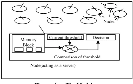
[image:3.595.322.551.601.746.2]Fourth, the final step, the algorithm generates a suspicion quotient to represent how suspicious this session is compared with all other sessions and a knowledge based system can take decision to expel the malicious node from the network opology. Our proposed model is shown in the Figure: 1
Figure: 1 The Model
Memory Block
Current threshold Decision
Block Nodes
Table: 1 Regression analysis & auto correlation coefficient.
4. RESULTS
As our processor utilization techniques is applicable to program or application running on any sensor node. The observed behaviour of a sensor node is done by first creating vectors to represent the activities of a particular node by monitoring the processor utilization for a time period of 0-69 seconds with interval of time 3seconds between two readings and the same process is repeated till the formation of the three different collected vectors generated represented by X1, X2 at different time T = <t1, t2, …, tn>. Processor utilization mean is calculated for each vectors and a range is formed. Table: 1 shows the regression analysis & auto correlation coefficient of the data obtained from different observations by the use of SPSS version 17.0. As in our data we have taken the significance level to be equal to 10 % hence according to that the X5 & X6 are not found to be significant because of their respective values i.e. 0.510 & 0.607; this shows that observations obtained for these variables are significant at 51% variables are significant at 51% & 60% respectively. And also it is important to note that these two variables are showing the problem of auto correlation as there coefficients i.e Durbin- Watson
coefficient have values less than the permissible level which shows that the values of these two variables are themselves auto correlated. Hence from this regression analysis & D-W analysis it is evident that variables X5 & X6 are not showing the perfect behaviour so it can be considered as malicious. Now this range describes the character of the processor for the particular application which we run. The range is stored in the profile of the node. We altered the code with repeating same of codes. Again we repeated the above described step and formed a vector and mean is calculated and compared with the threshold range. The results are as shown in the graph Figure: 2, vector X5 and X6 shows a significant deviation from the node’s expected behavior which flagged as a potential malicious. We again crosschecked our result by repeating the last step, which potentially confirm that the node is malicious the result are We also repeated the above steps by varying the time for monitoring the processor utilization from 0-10 sec with the interval of time 3 seconds and the end result shows a significant deviation from the node’s expected behavior which
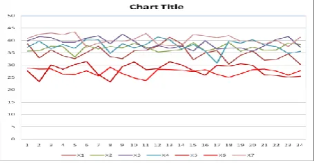
flagged as a potential malicious. Graphical representation v/s %CPU Utilization and Time as shown in
Figure 2 .It shows the actual behavior of a node for vectors X1, X2, X3, X4 and X5,X6 shows the malicious behavior of the sensor node after the modification in the code. From the data set in the present study, the efficiency score
processor utilization have been calculated using CSR model
of DEA technique of efficiency and performance measurement. The output maximization case has been considered to analyse the performance of the senor node processor. It has been experienced from the table 2 that the overall performance of the processor in different time period is 93.40 % , representing without altering the inputs. The output can be proportionally varied by 6.6 percent.
Further in time period 2nd, 5th 6th the processor is showing inefficient utilization. Therefore, there can be relative variation in the efficiency level by 0.9 percent, 19.0 percent and 26.1 percent without changing their input level. The reason for the inefficient performance of these processor utilization in their respective time period is due to alter in code .Therefore ,to attain the optimum efficient frontier ,they require to operate alike their
reference set as presented in the table 3 .it has been inferred from the table that the processor at time period 3 is having most number of reference counts ,there by depicting the most efficient utilization of the processor .The efficient processor utilization with wts λ’s aredefining the efficient points on the frontier for the inefficient ones .Thus inefficient processor utilization in different period are guided to produce their output by following the practice of their reference group.
[image:4.595.327.555.505.623.2]
Figure 2: Different collected vectors generated represented by X1, X2, X3, X4, X5, and X6
Model R R Square Adjusted R Square
Std. Error of the Estimate
R Square Change
F
Change df1 df2
Sig. F Change
R Square Change
F
Change df1 df2
Durbin-Watson
X1 0.309 0.095 0.054 20.63042 0.055 2.318 1 22 0.142 1.630
X2 0.248 0.062 0.019 21.01148 0.062 1.444 1 22 0.242 1.670
X3 0.462 0.213 0.178 19.23702 0.021 5.968 1 22 0.023 1.750
X4 0.21 0.044 0.001 21.20674 0.044 1.014 1 22 0.325 1.890
X5 0.105 0.011 -0.034 21.56932 0.510 0.247 1 22 0.624 0.036
X6 0.086 0.007 -0.038 21.60939 0.607 0.164 1 22 0.689 0.031
Table: 2 Performance of the processor in different time period
Table :3 Reference set
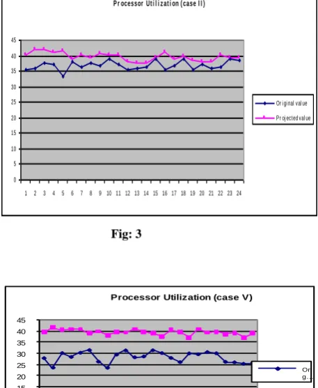
Thus, the projected point for this processor lies on joining points 7 and 3, defining the peer for the processor in time period 2.The projected points are the linear combinations of points 7 and 3 ,where the weights in the linear combinations are λ’s .Therefore for point 7 and 3 ,the reference weights are 0.560 and 0.440 ,employing that 56.0 percent of the processor in time period 7 are suitable for the processor in time period 1 and remaining 44.0 percent to be adopted from 3. The similar discussion could go for other inefficient processor utilization at different time period also. It also has been concluded from the table that the efficiency score equal to unity are references or bench mark for themselves. Figure 3, 4. and .5 represents the original and the projected values for the inefficient processors in time period 2and 6 .In case of time period 2, there is less deviation of the values
from the original ones, representing the less range of inefficiency than the processor in time period 5 and 6 .As in the case of 5 and 6 there has been alteration in the software before running in a particular time period .Consequently ,there is presence of more inefficiency in processor utilization in case 6 than in 5 .In order to perform it in a optimal level and to obtain the 100% processing utilization ,alteration in the code should be remove first before making them to operate again .
Fig: 3
Fig: 4
Fig: 5.
Time (in seconds)
DMUs
Technical Efficiency
120
0 i
i
t
1 1.000
120
0 i
i
t
1 0.991
120
0 i
i
t
1 1.000
120
0 i
i
t
1 1.000
120
0 i
i
t
(after alteration)
1 0.810
120
0 i
i
t
(after alteration)
1 0.739
120
0 i
i
t
1 1.000
Mean 0.934
unit Reference
set
Reference wt Reference count
1 1 1 1
1 7 3 0.56 0.4 0
1 3 1 3
1 4 1 2
1 7 3 4 0.55 0.1 0.366 0
1 7 3 1 4 0.92 0 0.002 0.366 0
1 7 3
P r ocessor Ut i l i z at i on ( case I I )
0 5 10 15 20 25 30 35 40 45
1 2 3 4 5 6 7 8 9 10 11 12 13 14 15 16 17 18 19 20 21 22 23 24
Or i gi nal val ue
Pr oj ected val ue
0 5 10 15 20 25 30 35 40 45
1 2 3 4 5 6 7 8 9 101112131415161718192021222324
Processor Utilization (case V)
Ori g…
P r oc e ssor U t i l i z a t i on ( VI )
0 5 10 15 20 25 30 35 40 45 50
1 2 3 4 5 6 7 8 9 10 11 12 13 14 15 16 17 18 19 20 21 22 23
[image:5.595.343.572.182.461.2]For calculating %age alteration in the code we use regression dummy technique. In regression analysis, a dummy variable is one that takes the values 0 or 1 to indicate the absence or presence of some categorical effect that may be expected to shift the outcome. For example, In our analysis, dummy variables are used to indicate the alteration in application and represented as a numerical value 0 and 1, where 1 without alteration in the application and 0 for with alteration in the application. The dummy regression method for the testing of
the application embedded on the sensor node for the reliability declaration of the software using the regression equation is given by Y=bo +b1 x Di ,where b0 is called the intercept and b1 is called the slope and Di is called the Dummy variables. Y=Bo +b1 x Di model B is intercept and D is slope, intercept indicate from where line start and slop shows elasticity of dependent variable with respect to independent variable. In the above table B=28.121 and D=8.7. D=8.78 shows that due to 100 % change processor utilization , there is 8.78% change in software correction. Here intercept and slope both are significant because calculated t- value is more both in case of slope and intercept. Tabulated t-value is 1.7109 where we take 5 % confidence interval. Here we have calculated t-value 67.759 and 14.944 which is much bigger than 1.7109.From results analysis there is 6.6% change in the processor utilization if there is 8.78% . alteration in the code of the application and further alteration there is respective processor utilization. Thus work presents an automatic approach for the detecting degradation in the software service quality base on the processor utilization .The ability to detect and test such degradation in an important approach for assessing the reliability of session oriented real time software. The advantage using this technique that it is a very straight forward approach for testing of nodes in real
environment. Fig: 6
5.
CONCLUSION
AND
RECOMMENDATION
The evaluation of processor utilization is complex task because many different input and output factors affect the processor utilization performance of sensor node. Some may prefer to evaluate the performance on the basis of outputs and other may prefer to understand how certain inputs variables, like power supply, input data from neighbor’s nodes, etc affect the power utilization as measured through output data.
Beyond processor utilization we also want to focus on the technical efficiency of a processor .We have presented a technique (based on the DEA) that enables to evaluate the technical efficiency of a senor processor .Because processor utilization depends upon incorporation of multiple inputs and output, the ability of DEA to allow for incorporation of multiple inputs and outputs into one efficiency measure, makes it a powerful tool .DEA strengthen our research by providing us a fuller picture by measuring all inputs and outputs, it also helps us to differentiate between the technical efficiency of malicious
node and non malicious node and provides a diagnostic information for improving the technical efficiency.
We also want to evaluate how much effective alteration in the code effects the processor utilization. We have presented a technique based on the Regression(Dummy Regression)) that enables us to evaluate the results, In Regression analysis ,a dummy variable is one that takes the values 0 and 1to indicate the absence or presence of some categorical effect that be expected to shift the outcome ,which is suitable powerful tools in our analysis .
This approach should appeal to software testing engineer and scientists who want to ensure the reliability of the sensor node in a real working environment to avoid the malicious working of a sensor node. In which data received from sensor node do not shows any malicious behavior/activity of a sensor node and thus one area of future research can be sensor node software testing in a real world environment.
TABLE :4
6. REFERENCES
[1] Song JianHua, Ma ChuanXiang :A reputation-based Scheme against Malicious Packet Dropping for Mobile Ad Hoc Network.
[2] Y-C. Hu, A. Perrig, and D. Johnson, “Wormhole Attacks in Wireless Networks,” IEEE JSAC,vol. 24, no. 2, Feb. 2006.
[3] Lee, B. Han, and M. Shin, “Robust Routing in Wireless Ad Hoc Networks,” 2002 Int’l. Conf.Parallel Processing Wksps., Vancouver, Canada, Aug. 18–21, 2002.
[4] P. Yi et al., “A New Routing Attack in Mobile Ad Hoc Networks,” Int’l. J. Info. Tech., vol. 11,no. 2, 2005.
[5] D. Raffo et al., “Securing OLSR Using Node Locations,” Proc. 2005 Euro. Wireless, Nicosia,Cyprus, Apr. 10–13, 2005.
[6] B. Kannhavong et al., “A Collusion Attack Against OLSR-Based Mobile Ad Hoc Networks,”IEEE GLOBECOM ’06.
[7] Waldir Riberio Pires Junior, Thiago H. de Paula Figueiredo Hao Chi Wong :Malicious Node Detection in Wireless Sensor Networks .
Model
Bvg Unstandardized
Coefficient
Standardized
Coefficient
B Std.
Error Beta t
Sig
1
(constant) 28.1 67.76 0
0
[8] Rashid Hafeez Khokhar, Md Asri Ngadi , Satria Mandala:A Review of Current Routing Attacks in Mobile Ad Hoc Networks
[9] C. Karlof and D. Wagner. Secure routing in wireless sensor network: Attacks and countermeasures. First IEEE International Workshop on Sensor Network Protocols and Applications May 2003
[10]Daniel-Ioan Curiac,Ovidiu Banias,Octavian Dranga: Malicious Node Detection in Wireless Sensor Network Using an Auto regression Technique
[11]C. Perkins, E. Belding-Royer, and S. Das, “Ad Hoc On demand Distance Vector (AODV)Routing,” IETF RFC 3561, July 2003.
[12]B. Kannhavong, H. Nakayama, Y. Nemoto, N. Kato, A. Jamalipour. A survey of routing attacks in mobile ad hoc networks. Security in wireless mobile ad hoc and sensor networks, October 2007, page, 85-91
[13]B. Kannhavong et al., “A Collusion Attack Against OLSR-Based Mobile Ad Hoc Networks,”IEEE GLOBECOM ’06.
[14]Z. Karakehayov, “Using REWARD to Detect Team Black-Hole Attacks in Wireless Sensor Networks,” Wksp. Real-World Wireless Sensor Networks, June 20–21, 2005.
[15]S. Kurosawa et al., “Detecting Blackhole Attack on AODV-Based Mobile Ad Hoc Networks by Dynamic Learning Method,” Proc. Int’l. J. Network Sec., 2006.
[16]D. Johnson and D. Maltz, “Dynamic Source Routing in Ad Hoc Wireless Networks,” Mobile Computing, T. Imielinski and H. Korth, Ed., pp. 153-81. Kluwer, 146.
[17] Jyoti Raju and J.J. Garcia-Luna-Aceves, “ A comparison of On-Demand and Table-Driven Routing for Ad Hoc Wireless etworks’,” in Proceeding of IEEE ICC, June 2000.
[18]Y-C. Hu, A. Perrig, and D. Johnson, “Wormhole Attacks in Wireless Networks,” IEEE JSAC, vol. 24, no. 2, Feb. 2006.
[19]C. Perkins and E Royer, “Ad Hoc On-Demand Distance Vector Routing,” 2nd IEEE Wksp. Mobile Comp. Sys. and Apps., 149.
[20]L. Qian, N. Song, and X. Li, “Detecting and Locating Wormhole Attacks in Wireless Ad Hoc Networks
Through Statistical Analysis of Multi-path,” IEEE Wireless Commun. And Networking Conf. ’05.
[21]D. Raffo et al., “Securing OLSR Using Node Locations,” Proc. 2005 Euro. Wireless, Nicosia, Cyprus, Apr. 10–13, 2005.
[22]K. Sanzgiri et al., “A Secure Routing Protocol for Ad Hoc Networks,” Proc. 2002 IEEE Int’l.Conf. Network Protocols, Nov. 2002.
[23]P. Yi et al., “A New Routing Attack in Mobile Ad Hoc Networks,” Int’l. J. Info. Tech., vol. 11,no. 2, 2005.
[24] http://spie.org/x8693.xml?ArticleID=x8693,Internet28 Feb 2011
[25]Vera, A. & Kuntz, L. (2007), Process-based organization design and hospital efficiency, Health Care Management Review, 32(1), 55-65.
[26]Bruner Rick E. The decade in online advertising :1994 2004.http://www.doubleclick.com/us/knowlwdge_central/ documents/REARSEH/dc_decaderinonline_0504.pdf2005 . Charnes A, Copper WW,Rhodes E, Golany B. A development study of data envelopment analysis in measuring the maintenance untis in the U.S. air forces. In: Thompson R, Thrall RM, editors. The annals of operations research , vol.2. Norwell, MA: Kluwer; 1985.p. 96-112.
[27]Ritu Lohtia, Naveen Donthu, and Idil Yaveroglu. “Evaluating the Efficiency of Internet Banner Ads,” Journal of Business Research, 60 (2007), 365-370.
[28] S. Meguerdichian, F. Koushanfar, G. Qu and M. Potkonjak, "Exposure In Wireless Ad-Hoc Sensor Networks," Computer Science Department, University of California, Los Angeles, Electrical Engineering and Computer Science Department, University of California, Berkeley, Electrical and Computer Engineering Department, University of Maryland, March 2002.
[29] H. Bau, N. F. DeRooij and B. Kloeck, Mechanical Sensors, Volume 7, Sensors: A Comprehensive Survey, John Wiley & Sons, USA, December 1993.