Study of Fuzzy based Classifier Parameter across
Spatial Resolution
Rakesh Dwivedi
Indian Institute of Technology,Roorkee, India
Anil Kumar
Indian Institute of Remote Sensing, Dehradun, India
S. K. Ghosh
Indian Institute of Technology,Roorkee, India
ABSTRACT
Classification and interpretation of satellite images are complex processes and that may be affected by various factors. Most fuzzy based soft classification techniques have been used to provide a more appropriate and accurate area estimation when fine, medium and coarse spatial resolution data are being used. Spatial resolution determines the spatial details on the Earth surface and greatly reduces the problem of mixed pixel. This paper examines the effect of weighting exponent „m‟ parameter of fuzzy c-means (FCM) and possibilistic c-mean (PCM) classifiers with respect to entropy, an uncertainty indicator for different extracted classes. This paper measures uncertainty variations across spatial resolution for different class extraction. Uncertainty can be defined as skepticism wherein entropy is an absolute indicator of an uncertainty. In this research work, fuzzy c-means (FCM) and possibilistic c-mean (PCM) classifiers have been used and entropy is computed to visualize the uncertainty. For this research work Resourcesat-1 (IRS-P6) data sets from AWIFS, LISS-III and LISS-IV sensors of same date have been used. Accuracy assessment of a classified image is an integral part of image classification and in this research two things were involved first optimization of weighting exponent „m‟, and computation of entropy. From the resultant Table 1, 2, 3, 4, 5, 6, 7 and 8 shows that the optimum values of „m‟ for FCM classifier on homogenous land cover classes are 2.9 and for heterogeneous classes are 2.7 where the membership values are varying from 0.8 to 0.9 with lesser entropy values, i.e. 0.35. Similarly for PCM classifier the optimum value of „m‟ for homogenous land cover classes are 3.2 and for heterogeneous classes are 3.0 where the membership values are varying from 0.8 to 0.9 with lesser entropy values, i.e. 0.78. In the second phase of study, to analyze the effect of uncertain pixels in FCM and PCM classifiers, Euclidean norm has been chosen for both the classifiers whereas the values of weighting exponent „m‟ varies from 1.1 to 4.0 for Sal forest, Eucalyptus plantation, water bodies, agriculture land with crop, agriculture moist land without crop, and agriculture dry land without crop. It is observed from the result Table 1, 2, 3, 4, 5, 6, 7 and 8, that uncertainty ratio is almost equal to referential value 2.585, for FCM and PCM classifiers using Euclidean norm. This reflects that fuzzy based soft classifiers FCM and PCM are producing higher classification accuracy with minimum level of uncertainty.
Keywords
Fuzzy c-Mean (FCM), Possiblistic c-Mean (PCM), Entropy
1.
INTRODUCTION
Remote sensing images contain a mixture of pure and mixed pixels. While digital image classification, however, a pixel is frequently considered as a unit belonging to a single land cover class. However, due to limited image resolution, pixels
often represent ground areas, which comprise by two or more discrete land cover classes. For this reason, it has been proposed that fuzziness should be accommodated in the classification procedure so that pixels may have multiple or partial class membership [10]. In this case, a measure of the strength of member-ship for each class is output by the classifier, resulting in a soft classification technique [23]. Also recent advances in supervised image classification have shown that conventional „hard‟ classification techniques, which allocate each pixel to a specific class, are often inappropriate for applications where mixed pixels are abundant in the image [8] & [9].
Mixed pixels are assigned to the class with the highest proportion of coverage to yield a hard classification. Due to which a considerable amount of information is lost. To overcome this loss, soft classification was introduced. A soft classification assigns a pixel to different classes according to the area it represents inside the pixel. This soft classification yields a number of fraction images equal to the number of land cover classes. Several researchers have addressed this soft mixture problem. Among the most popular techniques for soft classification are artificial neural networks [13], mixture modeling [14] and supervised fuzzy c-means classification [22]. [2], [3] and [6] used nonlinearity to fuzzify the crisp c-means. The method of [2], [6], and [18] has another feature: it smoothes the crisp solution into a differentiable one. Moreover this fuzzy solution approximates the crisp one in the sense that the fuzzy solution converges to the crisp solution as; m1
.
in this work. So in-house developed SMIC (Sub-pixel Multi-Spectral Image Classifier) System [16] & [17] having fuzzy and entropy based fuzzy classifier with accuracy assessment module for fraction images used in this research work.
2.
CLASSIFIERS
AND
ACCURACY
APPROACHES
Fuzzy c-Means (FCM) was originally introduced by [2]. In this supervised classification technique each data point belongs to a cluster to some degree that is specified by a membership grade, and the sum of the memberships for each pixel must be unity. This can be achieved by minimizing the generalized least - square error objective function given in Eq. (1),
21 1
( , )
N c m
m ij i j
i j A
J U V X x
(1)
where Xi is the vector denoting spectral response of a pixel i, x is the collection of vector of cluster centers xj,
ij is class membership values of a pixel, c and N are number of clusters and pixels respectively, m is a weighting exponent (1<m<
),which controls the degree of fuzziness,
2 i j A
X x
is the squared distance (dij) between Xi and xj, and is given in Eq. (2),
2
2 T
ij i j A i j i j
d X x X X A X X
(2)
where A is the weight matrix. Amongst a number of A-norms, three namely Euclidean, Diagonal and Mahalonobis norm, each induced by specific weight matrix, are widely used. The formulations of each norm are given in Eq. (3), [2],
1
1 j
j
A I Euclidean Norm
A D Diagonal Norm
A C Mahalonbis Norm
(3)
Where I is the identity matrix, Dj is the diagonal matrix having diagonal elements as the eigen values of the variance covariance matrix, Cj given in Eq.(4),
1
N
T
j i j i j
i
C X x X x
(4)
The class membership matrix
ij is obtained using Eq.(5)wherein 2
ik
d
is computed using Eq. (6),
1 2 1 2 1 1 ij m c ij k ik d d
(5) 2 2 1 c ik ij jwhere
d
d
(6)
In PCM, for a good classification is it expected that actual feature classes will have high membership value, while unrepresentative features will have low membership values [15]. The objective function, which satisfies this requirement, may be formulated as given in Eq.(7)
2
1 1 1 1
( , ) 1
N c c N
m m
m ij i j j ij
i j A j i
J U V X v
(7) µij is calculated from Eq. (5).
In Eq. (7) where
j is the suitable positive number, first termdemands that the distances from the feature vectors to the prototypes be as low as possible, whereas the second term
forces the
ij to be as large as possible, thus avoiding the trivial solution. Generally,
j depends on the shape and average size of the cluster j and its value may be computed as given in Eq.(8);2 1 1 N m ij ij i j N m ij i d K
(8)Where K is a constant and is generally kept as one. After this, class memberships,
ij are obtained as mentioned in Eq. (9); 1 2 1
1
1
ij m ij jd
(9)Soft Accuracy Assessment Approach: Entropy
In any closed system, the entropy of the system will either remain constant or increase. This is known as the second law of thermodynamics from where the concept of entropy evolves. In information technology entropy is measure of the uncertainty [5] & [7]. Entropy is a measure of disorder, or more precisely unpredictability [19]. This study usage entropy, as a special criterion for visualizing and evaluating the uncertainty of the classified results of FCM, and PCM classifiers. This criterion is able to purely and completely reflect the uncertainty from the classified image [4] & [11]. The entropy has been expressed by Eqn. (10);
1 2
( ) log
M i i i w w Entropy x x x
(10) " " .i
where M denotes no of classes and w
is the estimated membership function of class i for pixel x x
For high uncertainty, the calculated entropy (Eq.(10)) is high and inverse. Therefore this criterion can visualize the pure uncertainty of the classification results.
3.
STUDY AREA AND DATA USED
The study area is located near Pantnagar town between 28º 53‟ 57.12” N - 28 º 56‟ 31.22” N latitudes and 79 º 34‟ 22.92” E - 79 º 36‟ 35.27” E longitudes (Fig. 1).
ResourceSat-1 (IRS-P6), satellite is unique in providing multispectral data at different spatial resolution, while preserving the spectral information. In this research work, AWIFS, LISS-III and LISS-IV data sets from Re-sourceSat-1 (IRS-P6) satellite have been used as shown in Fig.(1). The fraction images and entropy would be used for the purpose of accuracy assessment.
LISS-IV LISS-III AWIFS Fig 1: Location of study area
4.
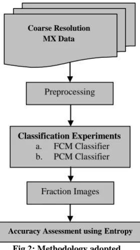
METHODOLOGY
and resampled using nearest neighbor resample method at 60m, 20m and 5m spatial resolution respectively to maintain the correspondence of a AWiFS pixel with specific number of LISS-III pixels (here 9, corresponding to AWIFS) as well as with LISS-IV pixels (here 144 pixels, corresponding to AWIFS) with respect to sampling during accuracy assessment.
[image:3.595.100.240.320.569.2]Training data set was collected from AWiFS, LISS-III and LISS-IV imageries with reference to toposheet of the same area. There are six information classes i. e. Sal forest, and Eucalyptus plantations are treated as a heterogeneous classes and agriculture land with crop, agriculture moist land without crop, agriculture dry land without crop, and water body classes are considered as a homogenous classes. For the purpose of experimentation, 40 pixels were selected as sample according to 10n rule [12] to train the classifiers. For accuracy assessment 100 pixels per class were randomly selected from corresponding images. The flow chart of the methodology adopted is shown in Fig. 2.
Fig 2: Methodology adopted
After pre-processing and training dataset collection the AWiFS image was separately classified by FCM and PCM algorithm using Euclidean norm. In this study a Euclidean distance measure that uses mean of the training class has been used for the spectral seperability analysis.
Euclidean Norm of weight matrix „A‟ in Eq.(3) has been taken, as it gives maximum classification accuracy compared to other weighted norms and less effected with noise outlier present in training data. As Euclidean Norm uses only mean value but other norms uses mean as well as variance-covariance. Mean is less affected than variance-covariance due to the presence of noise in training data [1] & [17]. The accuracy of classified imagery is validated using entropy. The use of entropy based accuracy assessment however provided an absolute uncertainty indication in the classified results.
5.
RESULTS AND DISCUSSIONS
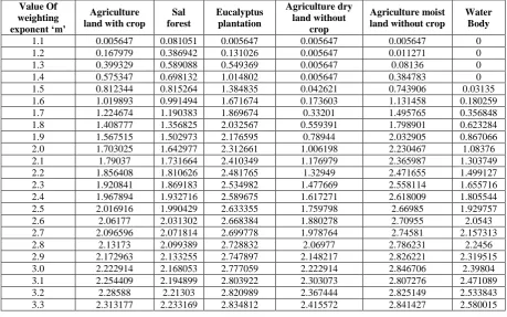
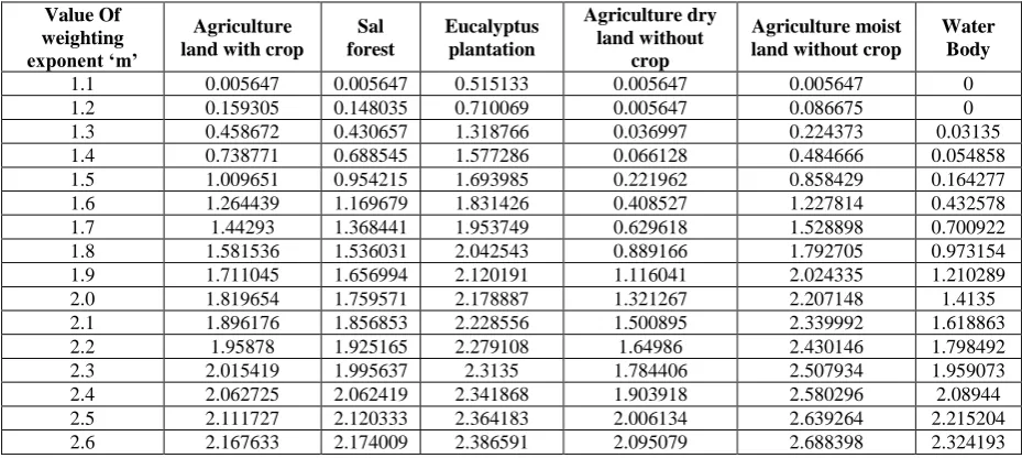
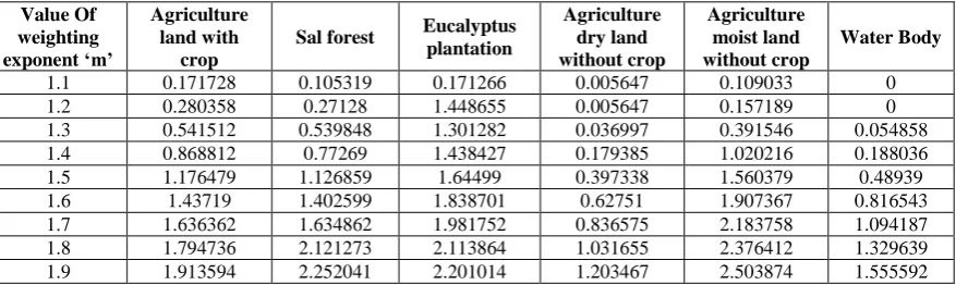
The uncertainty is a significant issue in the classification of remote sensing data. The uncertainty estimation of the classification results is important and necessary to evaluate the classifier performance. This study addresses the evaluation of entropy, based on FCM and PCM classifier which estimates uncertainty in classification results. In varying spatial resolution of classification and reference sub-pixel outputs entropy give the true reflectance of uncertainty ratio among various classes. The uncertainty criteria have been estimated from computed entropy based on actual output of classifier. To investigate the effect of uncertain pixels in FCM and PCM classifiers , Euclidean norm has been chosen for both the classifiers whereas the values of weighting exponent „m‟ varies from 1.1 to 4.0 for Sal forest, Eucalyptus plantation, water bodies, agriculture land with crop, agriculture moist land without crop, and agriculture dry land without crop. It is observed from the result Table 1, 2, 3, 4, 5, 6, 7 and 8, that uncertainty ratio is almost equal to referential value 2.585, for FCM and PCM classifiers using Euclidean norm. This reflects that fuzzy based soft classifiers FCM and PCM are producing higher classification accuracy with minimum level of uncertainty. The computation of entropy is an absolute reflector of an uncertainty and this study identifies that entropy criterion provides stable results for FCM and PCM, classifier for optimized value of „m‟.
For setting the optimized value of m, a number of experiments have been conducted individually for both classifiers by varying m from 1.1 to 4.0. It has been observed from the resultant Tables 1, 2, 3, 4, 5 and 6 that for homogenous classes like Agriculture land with crop, Agriculture dry land without crop Agriculture moist land without crop, and Water Body for FCM classifiers the optimized value of „m‟ is 2.9 and PCM classifiers this optimized value of „m‟ is 3.2. Similarly for heterogeneous classes like Sal forest and Eucalyptus plantation, the optimized value of „m‟ for FCM classifier is 2.7 and for PCM classifier is 3.0. These findings suggest that using these optimized values of „m‟ for FCM and PCM classifiers on homogenous and heterogeneous land cover classes the range of the computed entropy varies between the range of [0,3] as shown in resultant Tables 1 to 6. This in turn states that the information uncertainty is not exceeding more than 3%. In this research entropy has been used to measure the accuracy in terms of uncertainty without using any kind of ground reference data. This classification accuracy is directly measured by entropy. Measuring the spatial statistics of a satellite image using an entropy, of six land cover classes can be measured using Eq. (10) i. e. 6*(-1/6*log21/6)=2.585 [21]. This states that if the computed entropy values of classified images are lying within this range; then indirectly this reflects better classification results. It is shown in Table 1, 2, 3, 4, 5 and 6 where AWIFS, LISS-III and LISS-IV entropy of FCM and PCM classifiers for six land cover classes have been computed and, found that the entropy values are approximately lying within the specified range wherein the value of weighting exponent is lying from 1.1 to 4.0.
Preprocessing
Coarse Resolution MX Data
Classification Experiments a. FCM Classifier b. PCM Classifier
Fraction Images
Table 1. AWIFS entropy of various land cover classes from FCM classification output Value of
weighting exponent ‘m’
Agriculture land with crop
Sal forest
Eucalyptus plantation
Agriculture dry land without
crop
Agriculture moist land without crop
Water Body
1.1 0 0 0.005647 0 0.005647 0
1.2 0 0 0.005647 0 0.042621 0
1.3 0 0.005647 0.011271 0 0.07731 0
1.4 0.005647 0.005647 0.011271 0.005647 0.108948 0
1.5 0.005647 0.005647 0.011271 0.005647 0.201273 0
1.6 0.005647 0.005647 0.114217 0.011271 0.374569 0
1.7 0.011271 0.005647 0.219443 0.048223 0.607945 0.005647
1.8 0.042621 0.005647 0.372583 0.085153 0.827369 0.005647
1.9 0.048223 0.005647 0.50455 0.153411 1.059939 0.005647
2.0 0.07731 0.005647 0.696694 0.198918 1.321087 0.005647
2.1 0.108948 0.005647 0.889023 0.311619 1.49718 0.011271
2.2 0.155768 0.005647 1.025828 0.421707 1.631763 0.011271
2.3 0.229191 0.005647 1.189574 0.592181 1.740952 0.011271
2.4 0.2914 0.011271 1.323116 0.745557 1.849475 0.016873
2.5 0.349979 0.048223 1.450184 0.902941 1.955882 0.016873
2.6 0.429351 0.053802 1.536682 1.020398 2.01337 0.053802
2.7 0.499022 0.082867 1.628828 1.131156 2.081574 0.142274
2.8 0.528254 0.108948 1.718866 1.24783 2.12721 0.164456
2.9 0.640882 0.133084 1.800708 1.371942 2.171966 0.30079
3.0 0.751242 0.192584 1.883666 1.498588 2.228732 0.311653
3.1 0.800653 0.243009 1.940604 1.579978 2.263866 0.34832
3.2 0.891978 0.268888 1.994867 1.648406 2.283853 0.468001
3.3 0.979401 0.314408 2.046533 1.717386 2.319002 0.519514
3.4 1.060584 0.343834 2.094014 1.786385 2.335892 0.564537
3.5 1.157506 0.448557 2.134659 1.845735 2.353021 0.65343
3.6 1.221567 0.54316 2.149877 1.903476 2.38049 0.706779
3.7 1.30389 0.587018 2.176498 1.954026 2.388224 0.807428
3.8 1.340089 0.678095 2.216589 2.002838 2.407193 0.887616
3.9 1.431974 0.713617 2.250574 2.054258 2.425069 0.993425
4.0 1.477623 0.790351 2.252167 2.094103 2.424216 1.020262
Table 2. AWIFS entropy of various land cover classes from PCM classification output Value Of
weighting exponent ‘m’
Agriculture land with crop
Sal forest
Eucalyptus plantation
Agriculture dry land without
crop
Agriculture moist land without crop
Water Body
1.1 0.005647 0.081051 0.005647 0.005647 0.005647 0
1.2 0.167979 0.386942 0.131026 0.005647 0.011271 0
1.3 0.399329 0.589088 0.549369 0.005647 0.08136 0
1.4 0.575347 0.698132 1.014802 0.005647 0.384783 0
1.5 0.812344 0.815264 1.384835 0.042621 0.743906 0.03135
1.6 1.019893 0.991494 1.671674 0.173603 1.131458 0.180259
1.7 1.224674 1.190383 1.869674 0.33201 1.495765 0.356848
1.8 1.408777 1.356825 2.032567 0.559391 1.798901 0.623284
1.9 1.567515 1.502973 2.176595 0.78944 2.032905 0.867066
2.0 1.703025 1.642977 2.312661 1.006198 2.230467 1.08376
2.1 1.79037 1.731664 2.410349 1.176979 2.365987 1.303749
2.2 1.856408 1.810626 2.481765 1.32949 2.471655 1.499127
2.3 1.920841 1.869183 2.534982 1.477669 2.558114 1.655716
2.4 1.967894 1.932716 2.589675 1.617271 2.618009 1.805544
2.5 2.016916 1.990429 2.633355 1.759798 2.66985 1.929757
2.6 2.06177 2.031302 2.668384 1.880278 2.70955 2.0543
2.7 2.096596 2.071814 2.699778 1.978764 2.74581 2.157313
2.8 2.13173 2.099389 2.728832 2.06977 2.786231 2.2456
2.9 2.172963 2.133255 2.747897 2.148217 2.826221 2.319515
3.0 2.222914 2.168053 2.777059 2.222914 2.846706 2.39804
3.1 2.254409 2.194899 2.803922 2.303073 2.807276 2.471089
3.2 2.28588 2.21303 2.820989 2.367444 2.825149 2.533843
[image:4.595.68.528.481.768.2]3.4 2.333332 2.253543 2.8479 2.460965 2.857763 2.621677
3.5 2.359567 2.269023 2.860937 2.507254 2.863999 2.663224
3.6 2.378925 2.290968 2.87349 2.530244 2.877346 2.706939
3.7 2.402141 2.316157 2.885775 2.566049 2.881051 2.737986
3.8 2.425806 2.334049 2.894825 2.604207 2.891998 2.769042
3.9 2.444881 2.352773 2.902729 2.636352 2.902443 2.799337
[image:5.595.70.527.171.549.2]4.0 2.467058 2.376502 2.91509 2.66271 2.902668 2.829192
Table 3. LISS-III entropy of various land cover classes from FCM classification output Value Of
weighting exponent ‘m’
Agriculture land with crop
Sal forest
Eucalyptus plantation
Agriculture dry land without
crop
Agriculture moist land without crop
Water Body
1.1 0.005647 0.005647 0 0.005647 0.005647 0
1.2 0.005647 0.005647 0.005647 0.005647 0.011271 0
1.3 0.005647 0.005647 0.005647 0.005647 0.016873 0
1.4 0.005647 0.005647 0.005647 0.005647 0.022452 0
1.5 0.005647 0.005647 0.005647 0.005647 0.053802 0
1.6 0.042621 0.042621 0.005647 0.011271 0.23809 0
1.7 0.097857 0.07173 0.005647 0.053802 0.415129 0.005647
1.8 0.144767 0.127572 0.005647 0.193452 0.653195 0.005647
1.9 0.192398 0.192398 0.005647 0.330244 0.864063 0.005647
2.0 0.286224 0.280851 0.005647 0.530687 1.068206 0.005647
2.1 0.382887 0.371918 0.011271 0.726706 1.260592 0.011271
2.2 0.469436 0.450103 0.016873 0.902965 1.412865 0.022452
2.3 0.540047 0.517542 0.022452 1.068946 1.54625 0.033543
2.4 0.637522 0.580463 0.096244 1.218001 1.684216 0.11271
2.5 0.790682 0.639519 0.191075 1.360741 1.798627 0.238685
2.6 0.874402 0.731231 0.248428 1.48356 1.901779 0.368867
2.7 0.9576 0.811808 0.325234 1.581556 1.984885 0.449749
2.8 1.063631 0.949098 0.375461 1.668634 2.049721 0.548482
2.9 1.140056 1.099411 0.475092 1.740039 2.100816 0.642982
3.0 1.234354 1.211541 0.627877 1.825913 2.147537 0.735558
3.1 1.318565 1.315615 0.725852 1.838011 2.191935 0.840068
3.2 1.389581 1.413052 0.815275 1.898131 2.227696 0.967095
3.3 1.453251 1.500534 0.914436 1.955376 2.265943 1.077958
3.4 1.514214 1.583281 0.986734 2.003771 2.302689 1.178255
3.5 1.588201 1.653662 1.076588 2.058301 2.32652 1.273366
3.6 1.655488 1.717781 1.161803 2.103118 2.346336 1.353272
3.7 1.722504 1.766239 1.243087 2.15266 2.356008 1.430058
3.8 1.783701 1.800336 1.307944 2.193785 2.383625 1.487738
3.9 1.842241 1.814725 1.380038 2.230366 2.402686 1.555798
[image:5.595.65.530.560.768.2]4.0 1.857169 1.824889 1.423223 2.259975 2.402588 1.589166
Table 4. LISS-III entropy of various land cover classes from PCM classification output Value Of
weighting exponent ‘m’
Agriculture land with crop
Sal forest
Eucalyptus plantation
Agriculture dry land without
crop
Agriculture moist land without crop
Water Body
1.1 0.005647 0.005647 0.515133 0.005647 0.005647 0
1.2 0.159305 0.148035 0.710069 0.005647 0.086675 0
1.3 0.458672 0.430657 1.318766 0.036997 0.224373 0.03135
1.4 0.738771 0.688545 1.577286 0.066128 0.484666 0.054858
1.5 1.009651 0.954215 1.693985 0.221962 0.858429 0.164277
1.6 1.264439 1.169679 1.831426 0.408527 1.227814 0.432578
1.7 1.44293 1.368441 1.953749 0.629618 1.528898 0.700922
1.8 1.581536 1.536031 2.042543 0.889166 1.792705 0.973154
1.9 1.711045 1.656994 2.120191 1.116041 2.024335 1.210289
2.0 1.819654 1.759571 2.178887 1.321267 2.207148 1.4135
2.1 1.896176 1.856853 2.228556 1.500895 2.339992 1.618863
2.2 1.95878 1.925165 2.279108 1.64986 2.430146 1.798492
2.3 2.015419 1.995637 2.3135 1.784406 2.507934 1.959073
2.4 2.062725 2.062419 2.341868 1.903918 2.580296 2.08944
2.5 2.111727 2.120333 2.364183 2.006134 2.639264 2.215204
2.7 2.228392 2.220678 2.41137 2.177226 2.732176 2.423656
2.8 2.268899 2.266992 2.441783 2.26451 2.766897 2.50298
2.9 2.31079 2.316862 2.459165 2.343095 2.780304 2.576516
3.0 2.34609 2.355302 2.486786 2.407492 2.813747 2.638276
3.1 2.384577 2.392002 2.499265 2.470531 2.840047 2.691409
3.2 2.415658 2.417195 2.511218 2.529309 2.864499 2.737175
3.3 2.445378 2.441422 2.52796 2.577478 2.887159 2.777622
3.4 2.467903 2.465294 2.546082 2.622474 2.908079 2.811794
3.5 2.495519 2.487401 2.568461 2.656918 2.923335 2.843927
3.6 2.51675 2.509808 2.58812 2.682804 2.936682 2.874073
3.7 2.538504 2.53187 2.606685 2.710862 2.948797 2.902011
3.8 2.559757 2.55343 2.626424 2.734912 2.956965 2.930187
3.9 2.580511 2.57636 2.644617 2.764053 2.964735 2.950723
[image:6.595.74.522.247.611.2]4.0 2.60552 2.593914 2.658435 2.784166 2.975491 2.973742
Table 5: LISS-IV entropy of various land cover classes from FCM classification output Value Of
weighting exponent ‘m’
Agriculture land with
crop
Sal forest Eucalyptus plantation
Agriculture dry land without crop
Agriculture moist land without crop
Water Body
1.1 0.005647 0.005647 0.005647 0 0.005647 0
1.2 0.005647 0.005647 0.005647 0 0.073972 0
1.3 0.005647 0.122038 0.005647 0 0.294907 0
1.4 0.07173 0.261892 0.005647 0.005647 0.653681 0
1.5 0.144767 0.438321 0.005647 0.005647 1.05517 0
1.6 0.244104 0.585606 0.011271 0.005647 1.35955 0.005647
1.7 0.364689 0.714277 0.085153 0.005647 1.603583 0.005647
1.8 0.472074 0.850389 0.163806 0.011271 1.783335 0.011271
1.9 0.573062 0.980095 0.242081 0.053802 1.926197 0.016873
2.0 0.688359 1.154796 0.313409 0.187964 2.024459 0.059359
2.1 0.812223 1.271646 0.468849 0.308693 2.094082 0.162102
2.2 0.919235 1.385334 0.577848 0.436872 2.149881 0.277342
2.3 1.079375 1.466096 0.737814 0.558686 2.190752 0.382014
2.4 1.21204 1.562146 0.854526 0.697262 2.231481 0.531827
2.5 1.318114 1.653353 0.971561 0.826206 2.264671 0.64054
2.6 1.40474 1.730904 1.127387 0.947186 2.295833 0.765352
2.7 1.504222 1.801376 1.2389 1.061286 2.325257 0.870188
2.8 1.591054 1.867524 1.343727 1.208763 2.348919 0.995889
2.9 1.661768 1.918553 1.442624 1.335706 2.371786 1.104937
3.0 1.73146 1.968721 1.542677 1.42612 2.397596 1.225059
3.1 1.794947 2.016358 1.617287 1.492632 2.418438 1.331407
3.2 1.85302 2.05725 1.688421 1.584244 2.438308 1.416639
3.3 1.907959 2.09954 1.756235 1.664608 2.453257 1.491422
3.4 1.960115 2.139969 1.815458 1.732818 2.471248 1.566883
3.5 2.007936 2.179333 1.872325 1.807625 2.482828 1.63579
3.6 2.053551 2.213982 1.915535 1.867013 2.479834 1.698745
3.7 2.095712 2.244192 1.957011 1.91358 2.486553 1.765685
3.8 2.114165 2.262875 1.996795 1.960827 2.492935 1.843503
3.9 2.122742 2.26965 2.040745 2.011581 2.498988 1.897505
[image:6.595.81.520.634.765.2]4.0 2.124947 2.269793 2.061909 2.070317 2.504722 1.942477
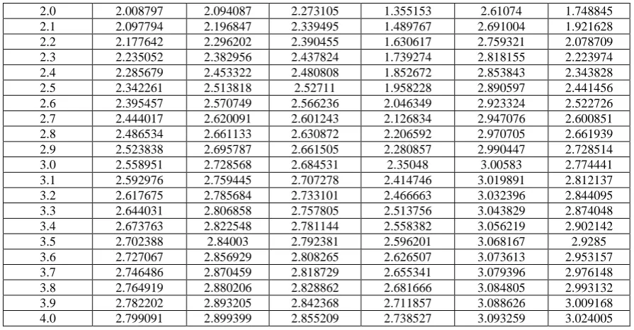
Table 6: LISS-IV entropy of various land cover classes from PCM classification output Value Of
weighting exponent ‘m’
Agriculture land with
crop
Sal forest Eucalyptus plantation
Agriculture dry land without crop
Agriculture moist land without crop
Water Body
1.1 0.171728 0.105319 0.171266 0.005647 0.109033 0
1.2 0.280358 0.27128 1.448655 0.005647 0.157189 0
1.3 0.541512 0.539848 1.301282 0.036997 0.391546 0.054858
1.4 0.868812 0.77269 1.438427 0.179385 1.020216 0.188036
1.5 1.176479 1.126859 1.64499 0.397338 1.560379 0.48939
1.6 1.43719 1.402599 1.838701 0.62751 1.907367 0.816543
1.7 1.636362 1.634862 1.981752 0.836575 2.183758 1.094187
1.8 1.794736 2.121273 2.113864 1.031655 2.376412 1.329639
2.0 2.008797 2.094087 2.273105 1.355153 2.61074 1.748845
2.1 2.097794 2.196847 2.339495 1.489767 2.691004 1.921628
2.2 2.177642 2.296202 2.390455 1.630617 2.759321 2.078709
2.3 2.235052 2.382956 2.437824 1.739274 2.818155 2.223974
2.4 2.285679 2.453322 2.480808 1.852672 2.853843 2.343828
2.5 2.342261 2.513818 2.52711 1.958228 2.890597 2.441456
2.6 2.395457 2.570749 2.566236 2.046349 2.923324 2.522726
2.7 2.444017 2.620091 2.601243 2.126834 2.947076 2.600851
2.8 2.486534 2.661133 2.630872 2.206592 2.970705 2.661939
2.9 2.523838 2.695787 2.661505 2.280857 2.990447 2.728514
3.0 2.558951 2.728568 2.684531 2.35048 3.00583 2.774441
3.1 2.592976 2.759445 2.707278 2.414746 3.019891 2.812137
3.2 2.617675 2.785684 2.733101 2.466663 3.032396 2.844095
3.3 2.644031 2.806858 2.757805 2.513756 3.043829 2.874048
3.4 2.673763 2.822548 2.781144 2.558382 3.056219 2.902142
3.5 2.702388 2.84003 2.792381 2.596201 3.068167 2.9285
3.6 2.727067 2.856929 2.808265 2.626507 3.073613 2.953157
3.7 2.746486 2.870459 2.818729 2.655341 3.079396 2.976148
3.8 2.764919 2.880206 2.828862 2.681666 3.084805 2.993132
3.9 2.782202 2.893205 2.842368 2.711857 3.088626 3.009168
4.0 2.799091 2.899399 2.855209 2.738527 3.093259 3.024005
6.
CONCLUSION
In this research work it has been tried to generate fraction outputs from FCM and PCM classifiers using Euclidean norm. These outputs have been generated from AWIFS, LISS-III and LISS-IV images of IRS-P6 data. Entropy has been used as assessment parameters of accuracy for various land cover classes i. e. water bodies, Sal forest, Eucalyptus plantation, agriculture land with crop, agriculture moist land without crop, agriculture dry land without crop. Uncertainty is intrinsic in spatial data and this generally refers to error, inexactness, fuzziness and ambiguity. The objective of this research on spatial data is to investigate, how uncertainties arise, or are created and propagated in the spatial data. Based on information theory, considering the characteristics of randomness of positional data and fuzziness of attribute data and taking entropy as a measure, this paper proposes the computational entropy model of spatial positional data uncertainty and fuzzy entropy model of spatial attribute data uncertainty. Usually, both randomness and fuzziness exist in spatial data simultaneously, so their co-uncertainty is also investigated and quantified in this paper. A novel spatial data uncertainty measure, total entropy, is presented. Total entropy can be used as a uniform measure to quantify the total spatial data uncertainty and fuzzy mixture uncertainty. In nutshell
[image:7.595.74.522.70.303.2] [image:7.595.78.522.71.303.2]this study on spatial variation has identified that total uncertainty which is not exceeding the referential value, 2.585; mentioned in Table 7 and 8 for any of the above mentioned six classes of homogenous and heterogeneous categories. This mathematical model of entropy computation is used as an absolute indicator of measuring uncertainty among various land cover classes, without using any ground reference data. Accuracy assessment of a classified image is an integral part of image classification and in this research two things were involved first optimization of weighting exponent „m‟, and computation of entropy. From the resultant table 1, 2, 3, 4, 5, 6, 7 and 8 shows that the optimum values of „m‟ for FCM classifier on homogenous land cover classes are 2.9 and for heterogeneous classes are 2.7 where the membership values are varying from 0.8 to 0.9 with lesser entropy values, i. e. 0.35. Similarly for PCM classifier the optimum value of „m‟ for homogenous land cover classes are 3.2 and for heterogeneous classes are 3.0 where the membership values are varying from 0.8 to 0.9 with lesser entropy values, i. e. 0.78. From the Table 7 and 8, it can be observed that at when the value of weighting exponent „m‟ is 4.0 the uncertainty is almost stable for all six land cover classes.
Table 7. Entropy variation for FCM Classifier Classifiers used for various
land cover classes
FCM Classifier
AWiFS Entropy LISS-III Entropy LISS-IV Entropy
Min Max Min Max Min Max
Agriculture land with crop 0 for m=1.1 1.47 at m=4.0 0 for m=1.1 1.85 at m=4.0 0 for m=1.1 2.12 at m=4.0 Sal forest 0 for m=1.1 0.79 at m=4.0 0 for m=1.1 1.82 at m=4.0 0 for m=1.1 2.26 at m=4.0 Eucalyptus plantation 0 for m=1.1 2.25 at m=4.0 0 for m=1.1 1.42 at m=4.0 0 for m=1.1 2.06 at m=4.0 Agriculture dry land without crop 0 for m=1.1 2.09 at m=4.0 0 for m=1.1 2.25 at m=4.0 0 for m=1.1 2.07 at m=4.0 Agriculture moist land without crop 0 for m=1.1 2.42 at m=4.0 0 for m=1.1 2.40 at m=4.0 0 for m=1.1 2.50 at m=4.0 Water Body 0 for m=1.1 1.02 at m=4.0 0 for m=1.1 1.58 at m=4.0 0 for m=1.1 1.94 at m=4.0
Table 8. Entropy variation for PCM Classifier Classifiers used for various
land cover classes
PCM Classifier
AWiFS Entropy LISS-III Entropy LISS-IV Entropy
[image:7.595.45.555.577.757.2]Agriculture land with crop 0 for m=1.1 2.46 at m=4.0 0 for m=1.1 2.60 at m=4.0 0.17 for m=1.1 2.79 at m=4.0 Sal forest 0 for m=1.1 2.37 at m=4.0 0 for m=1.1 2.59 at m=4.0 0.10 for m=1.1 2.89 at m=4.0 Eucalyptus plantation 0 for m=1.1 2.91 at m=4.0 0.5 for m=1.1 2.65 at m=4.0 0.17 for m=1.1 2.85 at m=4.0 Agriculture dry land without crop 0 for m=1.1 2.66 at m=4.0 0 for m=1.1 2.78 at m=4.0 0 for m=1.1 2.73 at m=4.0 Aggri. moist land without crop 0 for m=1.1 2.90 at m=4.0 0 for m=1.1 2.97 at m=4.0 0 .10 for m=1.1 3.09 at m=4.0 Water Body 0 for m=1.1 2.82 at m=4.0 0 for m=1.1 2.97 at m=4.0 0 for m=1.1 3.02 at m=4.0
7.
REFERENCES
[1] Aziz, M. A. 2004. “Evaluation of soft classifiers for remote sensing data”, unpublished Ph.D. thesis, IIT Roorkee, Roorkee, India.
[2] Bezdek, J. C. 1981. “Pattern Recognition with Fuzzy Objective Function Algorithms”, Plenum, New York, USA.
[3] Binaghi, E., Brivio, P. A., Chessi, P. and Rampini, A. 1999. “A fuzzy Set based Accuracy Assessment of Soft Classification”, Pattern Recognition letters, Vol. 20, 935-948.
[4] Congalton R. G. 1991. “A review of assessing the accuracy of classification of remotely sensed data”. Remote Sensing Environment, Vol. 37, 35-47, [doi:10.1016/0034-4257(91)90048-B.
[5] Dehghan H. and Ghassemian H. 2006. “Measurement of uncertainty by the entropy: application to the classification of MSS data”. International Journal of Remote Sensing, 1366 - 5901, Vol. 27, Issue 18, 4005 – 4014.
[6] Dunn J. C. 1973. “A Fuzzy Relative of the ISODATA Process and Its Use in Detecting Compact Well-Separated Clusters”, Journal of Cybernetics Vol. 3, 32-57.
[7] Foody G. M. 1995. “Cross-entropy for the evaluation of the accuracy of a fuzzy land cover classification with fuzzy ground data.” ISPRS Journal of Photogrammetry and remote sensing, Vol. 50, 2-12.
[8] Foody, G. M. 1996. “Approaches for the production and evaluation of fuzzy land cover classifications from remotely sensed data.” International Journal of Remote Sensing, Vol. 17, No. 7, 1317-1340.
[9] Foody, G. M. and Arora, M. K. 1996. “Incorporating mixed pixels in the training, allocation and testing stages of supervised classification,” Pattern Recognition Let-ters, Vol. 17, 1389-1398.
[10] Foody, G. M., Lucas, R. M., Curran, P. J. and Honzak, M. 1997. “Non-linear mixture modelling without end-members using an artificial neural network.” Inter-national Journal of Remote Sensing, Vol. 18, No. 4, 937-953.
[11]Goodchild M. F. 1995. “Attribute accuracy. In: Guptill S. C. and Morrison J. L. (eds), Elements of Spatial Data Quality (Elesevier Scientific, Oxford, 1995), 59–79. [12]Jensen, J. R. 1996. “Introductory Digital Image
Processing:” A Remote Sensing Perspective – 2nd edition (USA: Prentice Hall PTR).
[13]Kanellopoulos, I., Varfis, A., Wilkinson, G. G. and
HRV imagery using an artificial neural network:” a 20-class experiment. International Journal of Remote Sensing, Vol. 13, No.5, 917-924.
[14]Kerdiles, H. and Grondona, M. O. 1996. “NOAA-AVHRR NDVI decomposition and subpixel classification using linear mixing in the Argentinean Pampa”. International Journal of Remote Sensing, Vol. 16, No. 7, 1303- 1325.
[15]Krishnapuram, R., and Keller J., M. 1993. “A possibilistic approach to clustering”, IEEE Transactions on Fuzzy Systems, Vol. 1, 98-108.
[16]Kumar, A., Ghosh, S. K. and Dadhwal, V. K. 2005. “Advanced Supervised Soft Multi-Spectral Image Classifier,” Map Asia 2005 conference, Jakarta. Indonesia.
[17]Kumar, A., Ghosh, S. K., and Dadhwal V. K. 2006. “A comparison of the performance of fuzzy algorithm versus statistical algorithm based sub-pixel classifier for remote sensing data.” Proceedings of mid-term symposium ISPRS, ITC-The Netherlands.
[18]Okeke, F. and Karnieli, A. 2006. “Methods for fuzzy classification and accuracy assessment of historical aerial photographs for vegetation change analysis.” Part I: Algorithm development. International Journal of Remote Sensing, Vol.27, No. 1-2, 153-176.
[19]Shannon, C. E. 1948. “A mathematical theory of communication," Bell Syst. Tech. J. 623-656.
[20]Shi, W., Z., Ehlrs, M., and Temphli, K. 1999. “Analysis modeling of positional and thematic uncertainty in integration of remote sensing and GIS”, Transaction in GIS, Vol. 3, 119-136.
[21]Stein, A., Meer, F. V. D. and Gorte B. 2002. “Spatial Statistics for Remote Sensing,” 1st edition, Kluwer Academic Publishers, Netherlands.
[22]Verhoeye J. and Robert D. W. 2000. “Sub-pixel Mapping of Sahelian Wetlands using Multi-temporal SPOT Vegetation Images. Laboratory of Forest Management and Spatial Information Techniques,” Faculty of Agricultural and Applied Biological Sciences, University of Gent.
[23]Yannis, S. A., and Stefanos, D. K. 1999. “Fuzzy Image Classification Using Multi-resolution Neural with Applications to Remote Sensing.” Electrical Engineering Department, National Technical University of Athens, Zographou 15773, Greece.