Multi-Objective Constrained Optimization using
Discrete Mechanics and NSGA-II Approach
Sneha Desai
M.Tech Control System Department of Electrical Engineering, Veermata Jijabai Technological Institute (VJTI), INDIASushant Bahadure
M.Tech Control System Department of Electrical Engineering, Veermata Jijabai Technological Institute (VJTI), INDIAFaruk Kazi
Faculty at Department of Electrical Engineering Veermata Jijabai Technological Institute (VJTI), INDIA
Navdeep Singh
Faculty at Department of Electrical Engineering Veermata Jijabai Technological Institute (VJTI), INDIA
ABSTRACT
A novel approach to solve multi-objective optimization problems of complex mechanical systems is proposed based on evolution-ary algorithm. Discrete mechanics derives structure preserving con-straint equations and objective functions. Standard non-linear opti-mization techniques used to obtain optimal solution to these equa-tions fails to find global optimum solution and also requires system satisfying initial guess. Multi-objective optimization technique like non-dominated sorting genetic algorithm-II (NSGA-II) finds global optimal solution without giving any initial guess for multiple con-flicting objectives. This method is numerically illustrated by opti-mizing an underactuated mechanical system called 2D SpiderCrane system. In SpiderCrane, fast and precise payload positioning is to be achieved while keeping payload swing minimum along the tra-jectory. Minimizing the time of operation requires greater amount of force which may lead to unacceptable payload sway, while de-creasing forces increases the time of operation. Proposed control law to optimize this conflicting multi-objectives is validated with simulation results.
Keywords:
Optimization, Non-dominated sorting genetic algorithm, Dis-crete mechanics optimal control, Bio-inspired 2D Spider-Crane.ifx
1. INTRODUCTION
In order to solve multi-objective optimization problem of me-chanical systems, one is often interested in preserving certain properties of the mechanical system for the approximated so-lution and steer a mechanical system from an initial to a fi-nal state under the influence of control forces such that a given quantity, for example control effort or maneuver time is min-imal i.e multiple conflicting objectives are needed to be opti-mized. The presence of these multiple conflicting objectives for-mulates the task as a (global) multi-objective optimization prob-lem (MOP), which resorts to a number of trade-off optimal so-lutions. Classical methods like the objective weighted method, the hierarchical optimization, the constraint method, the goal programming method and many more aggregates the multiple-objective in a single, parametrized multiple-objective function. However, for systematically varying the parameters, knowledge of problem is very much necessary which may not be available [1]. Also, there are possibilities of producing biased result by setting pri-orities to objectives and finding one solution in one simulation run. Because of which several optimization runs are required to obtain approximate Pareto-optimal set. Evolutionary algorithms (EAs), on the other hand, can find multiple optimal solutions
in one single simulation run due to their population-approach. EAs are ideal for solving multi-objective optimization problems. Although there exist a number of multi-objective evolutionary algorithms (EMO), non-dominated sorting genetic algorithm II (NSGA-II), have gained tremendous popularity in solving differ-ent kinds of engineering problems [1], [2]. NSGA-II implemdiffer-ents elitism for multi-objective search which enhances the conver-gence properties towards the true Pareto-optimal set. The con-straint handling method does not make use of penalty parame-ters. The algorithm implements a modified definition of domi-nance in order to solve constrained multi-objective efficiently. Discrete Mechanics and Optimal Control (DMOC) is used to derive structure preserving constraint equations and objective functions. These equations are then used by NSGA-II to obtain global optimum solution. DMOC is introducesd in [4], [5]. In the context of variational integrators [6], the discretization of the Lagrange-d’Alembert principle leads to structure preserving time stepping equations which serve as equality constraints for the resulting finite dimensional non-linear optimization problem. This problem can be solved by standard non-linear optimization techniques such as Sequential Quadratic Programming (SQP) leading to local optimal solutions dependent on the initial guess [7]. Although this method works very successfully in many ap-plications, they fail to find the global optimal solution for MOP without using any initial guess. A remedy for these difficulty is found in the MOEA.
2. DISCRETE MECHANICS OPTIMAL CONTROL (DMOC)
In order to locally solve optimal control problems, DMOC is used which relies on a direct discretization of the variational for-mulation of the system dynamics. For convenience, we briefly summarize the basic idea, the more elaborate discussion can be found in [11], [4].
A mechanical system with configuration spaceMis to be moved on a curvex(t)∈M, t∈[0, T],form an initial state(q0,q˙0)to a final state(qT,q˙T)under the influence of a forcef:T M×U→
T∗M,whereT MandT∗Mare the tangent and cotangent space
of the configuration spaceM, respectively. This force depends on a time-dependent control effortu(t)∈U. The curvesqand ushall minimize a given objective functionalJ:T M×U →R
J(q,q, u˙ ) =
Z T
0
C(q(t),q˙(t), u(t))dt (1)
with the cost functionC :T M ×U → R.IfL :T M → R denotes the Lagrangian of the system, its motionq(t)satisfies theLagrange-d’Alembert principle,which requires that
δ ZT
0
L(q(t),q˙(t))dt+
Z T
0
f(q(t),q˙(t), u(t))dt= 0 (2)
for all variationsδqwithδq(0) = δq(T) = 0.This principle leads to a system of second order differential equations denoted as theforced Euler-Lagrange equations
d dt
∂ ∂q˙L(q,q˙)
− ∂
∂qL(q,q˙) =f(q,q, u˙ ) (3)
Final state is given by final time constraint r(q(t),q˙(t), qT,q˙T) = 0 with r : T M × T M →
Rnr, where (qT,q˙T) ∈ T M is fixed for desired final state. The minimization of (1) subject to the equations (3) and initial and final state conditions constitutes the optimal control problem in the continuous setting. Formulation of optimal control problem for a Lagrangian system is as follows:
Minimise cost functionJ
min
(q(·),q˙(·),u(·),T)
J(q,q, u˙ ) =
T
Z
0
C(q(t),q˙(t), u(t))dt, (4)
subjected to
δ
T
Z
0
L(q(t),q˙(t))dt+
T
Z
0
fLC(q(t),q˙(t), u(t))·δq(t)dt= 0,
q(0) =q0,q˙(0) = ˙q0,
h(q(t),q˙(t), u(t))≥0,
r(q(T)),q˙(T), qT,q˙T) = 0.
In this paper, we pose our optimization problem as moving the payload from an initial position to a given desired position with minimum swing, time and minimum control effort. Here, initial and final positions of the payload are considered as fixed bound-ary conditions.
Fixed Boundary Conditions. This is the special case of opti-misation problem with fixed initial and final velocities and con-figuration without path constraints,
min
q(·),q˙(·),u(·)J(q,q, u˙ ) = T
Z
0
C(q(t),q˙(t), u(t))dt, (5)
subjected to
δ
T
Z
0
L(q(t),q˙(t))dt+
T
Z
0
fLC(q(t),q˙(t), u(t))·δq(t)dt= 0,
q(0) =q0,q˙(0) = ˙q0, q(T) =qT,q˙(T) = ˙qT.
2.1 Discretization
During discretization the state spaceT Mof the continuous sys-tem is replaced byRand consider the grid∆t={tk=kh|k=
0, ..., N}, N h = T,whereN is a positive integer andhthe step size. The path q : [0,1] → Q is replaced by discrete pathqd : [0, h,2h, ...,(N h = 1)] → M.Similarly continu-ous forcef : [0,1]→ T∗M is approximated by discrete force
fd: [0, h,2h, ...,(N h= 1)]→T∗M.
Notations usedqk = qd(kh) andfk = fd(kh). An approx-imation of the action integral in (2) over small time interval
[kh,(k+ 1)h], by a discrete Lagrangian Ld : Q×Q → R yields
Ld(qk, qk+1)≈ (k+1)h
Z
kh
L(q(t),q˙(t))dt, (6)
anddiscrete forcesexpressed as
fk−·δqk+fk+·δqk+1≈ (k+1)h
Z
kh
f(q(t),q˙(t), u(t))·δq(t)dt, (7)
wherefk− and fk+ ∈ T∗Q are called left and right discrete
forcesrespectively. Now depending on(qk, qk+1, uk),the dis-crete Lagrange-d’Alembert principleis obtained in (8). This re-quires to find discrete paths{qk}Nk=0such that for all variations
{δqk}Nk=0withδq0=δqN= 0,one has
δ
N−1 X
k=0
Ld(qk, qk+1) + N−1 X
k=0 f−
k ·δqk+fk+·δqk+1= 0. (8)
which is equivalent to theforced discrete Euler-Lagrange equa-tions
D2Ld(qk−1, qk) +D1Ld(qk, qk+1) +fk+−1+f
−
k = 0, (9)
where k = 1,2, ..., N − 1, Di denotes the derivative w.r.t. the ith slot. In the same manner approximation of the objec-tive functional (1) is done and thediscrete objective functional Jd(qd, ud),is obtained such that theDiscrete Constrained Opti-mization Problemis
minqd,udJd(qd, ud) =
N−1 X
k=0
Cd(qk, qk+1, uk) (10)
subject to the discretized boundary constraints and the discrete Euler-Lagrange equations (9).
Discrete Cost Function. Approximation of the cost functional in short interval of time[kh,(k+ 1)h]is given as
Cd(qk, qk+1, uk)≈ (k+1)h
Z
kh
C(q(t),q˙(t), u(t))dt (11)
results in discrete cost function
Jd(qd, ud) = N−1 X
k=0
In our case we select the following cost function.
J1d(ud) = N
X
k=0
u2k, J2d(θd) = N
X
k=0
θ2k, (13)
J3d=Total time required for operation=T The cost function depends on the forces, Theta (θ) and T.
Boundary Conditions. All the initial and final conditions, configurations and velocities need to be assigned in discrete form in discrete fixed boundary optimisation problem.q(0) =
q0,q˙(0) = ˙q0andq(1) = q1,q˙(1) = ˙q1 as initial condition. q(N−1) =qN−1,q˙(N−1) = ˙qN−1andq(N) =qN,q˙(N) =
˙
qNthese two points lead to two discrete boundary conditions as discussed in [12] usingstandard Legendre transformation
D2L(q0,q˙0) +D1Ld(q0, q1) +f0−= 0, (14)
−D2L(qN,q˙N) +D2Ld(qN−1, qN) +fN+−1= 0. (15) Equation (14) is applied to initial discrete point and at final point (15) is applied. Equation (14) and (15) describes a non-linear optimization problem with equality constraints, which can be solved by standard optimization methods. With a local solver, for example, the SQP-method, one can find a local optimum. The initial guess of the optimization is chosen in a simple way. SQP is an iterative method for non-linear constrained optimization, used on problems for which the objective function and the constraints are twice continuously differentiable.
2.2 Advantages of The Proposed Approach
The SQP method used alongwith DMOC [13], have some no-table drawback:
1. SQP is local optimal solver so the obtained result is not the global optimal solution.
2. It is a single objective problem.
3. This technique requires an excellent initial guess and the rate of convergence of the solution are very sensitive to these guesses. The wrong selection of initial guess misleads the search.
To overcome the above drawbacks, Multi-objective optimization techniques like NSGA II can be used in place of SQP. The ad-vantages of Evolutionary techniques are as follows:
1. They are population based search algorithms, so global op-timal solution is possible. Population-based search techniques give multi-directional search. Therefore, they search whole so-lution space for global optimum soso-lution.
2. Optimizing all the objectives simultaneously and generating a set of alternative solutions offers more flexibility. The si-multaneous optimization can fit nicely with population-based approaches such as EAs, because they generate multiple solu-tions in a single run.
3. In case of population-based techniques, the final solution does not depend on the initial guess.
3. NON-DOMINATED SORTING GENETIC
ALGORITHM-II (NSGA-II)
A single objective optimization algorithm mostly terminates upon obtaining an optimal solution. In a typical multi-objective optimization problem, there exists a family of equivalent solu-tions that are superior to the rest of the solusolu-tions and are con-sidered equal from the perspective of simultaneous optimization of multiple conflicting objective functions. Such solutions are called non-inferior, non-dominated or Pareto-optimal solutions,
and are such that no objective can be improved without degrad-ing at least one of the others, and, given the constraints of the model, no solution exist beyond the true Pareto front.
[image:3.595.52.283.95.156.2]The goal of NSGA-II actually consists of two parts as mentioned in [1], namely that the solutions found must be: (i) close to the Pareto-optimal front, and (ii) diverse. This is also illustrated in Fig 1, where it is clear how solutions near the Pareto-optimal front are first obtained followed by a search for diversity along the front. The first requirement is obtained by using the dom-inance concept and does not have a need for any niching or crowding measures. Therefore, a good algorithm can find a set of solutions as close to the Pareto-optimal front as possible. How-ever, the second requirement can be more difficult to obtain. In order to obtain a diverse set, it must be specified what can be considered as a set of diverse solutions, but it must also be un-derstood how dominance has influenced the diversity of the so-lutions.
Fig. 1. Pareto-front and Non-domination illustration
The NSGA proposed by Srinivas and Deb (1994) has been suc-cessfully applied to solve many problems, the main criticisms of this approach has been its high computational complexity of non-dominated sorting, lack of elitism, and need for specifying a tunable parameter called sharing parameter [14]. Recently, Deb et al. reported an improved version of NSGA, which they called NSGA-II, to address all the above issues [2].
NSGA-II only differs from a simple genetic algorithm in the selection process. The population is initialized as usual. Once the population in initialized NSGA-II sorts the population based on non-domination into each front. The first front is completely non-dominant set in the current population and the second front is dominated only by the individuals in the first front and the front goes so on. Each individual in the each front are assigned rank (fitness) values based on front in which they belong to. Indi-viduals in first front are given a fitness value of 1 and indiIndi-viduals in second are assigned fitness value as 2 and so on. In addition to fitness value a new parameter called crowding distance is cal-culated for each individual. The crowding distance is a measure of how close an individual is to its neighbours. Large average crowding distance means better diversity in the population. Par-ents are selected from the population by using tournament selec-tion based on the rank and crowding distance. When comparing two individual, an individual belonging to lesser rank is given priority but if both individual have same rank, extreme individ-uals prevails over not extreme ones. If both individindivid-uals are not extreme, the one with the bigger crowding distance wins. The se-lected population then generates off-springs from crossover and mutation operators.
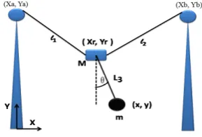
[image:3.595.349.503.290.389.2]4. 2D SPIDERCRANE
The proposed method is applied to 2D SpiderCrane system. Spi-derCrane is a pulley-cable system and cable systems are gener-ally underactuated which works on tensile forces. This system is similar to pendulum on a cart system where pendulum swing is non actuated. SpiderCrane is a crane designed to reduce the time required, for carrying loads, consider the 2D SpiderCrane mechanism as illustrated in Fig 2 [8].
[image:4.595.353.492.103.208.2]Crane operators moves the load in such a way that cable by which load is attached remains vertical for safety reasons, this strategy induces large economical loss due to additional time in-volved in process. To improve work rate one should anticipate swing of the load. The problem is to achieve fast and precise payload positioning while minimizing the swing. This problem has been approached by various control strategies [15]-[19].
Fig. 2. 2D SpiderCrane mechanism
In this model, the problem is to find the optimum effort path of the payload of massmsuspended by the cable from the ring of massM on which the actuating forcesFxandFyare applied. This type of analysis of the 2D SpiderCrane is termed as decou-pled SpiderCrane. The configuration variables for gantry crane mechanism are
q= (Xr,Yr, θ)T (16)
and Lagrangian may be defined as
L(q,q˙) =1 2q˙
TM(q) ˙q−V(q)
(17)
where,
M(q) =
(M+m) 0 mL3cosθ
0 (M+m) mL3sinθ ml3cosθ mL3sinθ mL23
(18)
and
V(q) = (M+m)gYr−mgL3cosθ (19)
The resulting Euler-Lagrange equations are:
Fx= (M+m) ¨Xr+ (mL3cosθ)¨θ−(mL3sinθ) ˙θ2 (20)
Fy= (M+m) ¨Yr+(mL3sinθ)¨θ+(mL3cosθ) ˙θ2+(M+m)g (21)
0 = (mL3cosθ) ¨Xr+ (mL3sinθ) ¨Yr+ (mL23)¨θ+mgL3sinθ (22) As from Fig 3,FxandFyare control forces applied on the ring of massMon which payload of massmis suspended with non elastic cable. This subsystem is referred asgantry mechanism ordecoupled SpiderCrane, where pulleys, cables and pylons are neglected for simplicity.
Fig. 3. Decoupled SpiderCrane model
4.1 Discretization
In this paper, a midpoint rule for integral approximation and derivative approximation over small intervalshis considered as follows
(k+1)h
Z
kh
f(x)dx≈hf(a+b 2 ).
We obtain velocity vector according to midpoint rule,
(qk+1−qk)
h ≈q˙
and position vector approximation according to midpoint rule,
qk+1+qk
2 ≈qk
as well as in case for discrete forces, we obtain
(k+1)h
Z
kh
f(t).δq(t)dt≈hfk+1+fk
2 .
δqk+1+δqk
2
=h
4(fk+1+fk).δqk+
h
4(fk+1+fk).δqk+1, (23)
i.e.fk−=fk+=h 4(f
k
k+1)were used as the left and right discrete forces. Discrete Lagrange is equivalent to continuous Lagrange
Ld(qk, qk+1) =hL
qk+1+qk
2 ,
qk+1−qk
h
, (24)
Using (17), (18), (19) and (24) Lagrangian is defined as
L=1
2[(M+m)( ˙Xr
2
+ ˙Yr 2
) + 2 ˙Xr 2˙
θ(mL3cosθ)
+2 ˙Yr 2
˙
θ(mL3sinθ) + ˙θ2(mL23)]−(M+m)gYr+mgL3cosθ
discrete Lagrangian is,
Ld(qk, qk+1)
=h
2(((M+m)[((Xrk+1−Xrk)/h)
2+ ((Y
rk+1−Yrk)/h)
2])
+2((Xrk+1−Xrk)/h)(θk+1−θk/h)(mL3cos((θk+1+θk)/2))
+2((Yrk+1−Yrk)/h)((θk+1−θk)/h)(mL3sin((θk+1+θk)/2))
+((θk+1−θk)/h)2(mL23))−(M+m)g((Yrk+1+Yrk)/2)
[image:4.595.94.239.282.380.2]Ld(qk−1, qk)
=h
2(((M+m)[((Xrk−Xrk−1)/h) 2+ ((Y
rk−Yrk−1)/h) 2])
+2((Xrk−Xrk−1)/h)(θk−θk−1/h)(mL3cos((θk+θk−1)/2))
+2((Yrk−Yrk−1)/h)((θk−θk−1)/h)(mL3sin((θk+θk−1)/2))
+((θk−θk−1)/h)2(mL23))−(M+m)g((Yrk+Yrk−1)/2)
+mgL3cos((θk+θk−1)/2) (26)
and discrete cost function as
Cd(fk, fk+1) =hC(
fk+1+fk
2 ). (27)
In this 2D SpiderCrane problem as seen from (20) and (21) ac-tuating discrete forcefkcan be represented as
uk=fk=
Fxk Fyk
(28)
Now from (13) and (27) discrete cost function for 2D Spider-Crane can be formulated. Since we formulated our problem as constrained optimization problem, Forced discrete Euler La-grange equation (9) and discrete boundary condition (14) and (15) serves as constraints and are as follows.
Constraint for initialθ,
(M+m)((θ(2)−θ(1))/h) + ((mL)cos((θ(2) +θ(1))/2) ((Yr(2)−Yr(1))/h)) +h(((M+m)((θ(2)
−θ(1))/h)(−1/h)) + (((mL)((Yr(2)
−Yr(1))/h))((cos((θ(2) +θ(1))/2)(−1/h))
+(((θ(2)−θ(1))/h)sin((θ(2) +θ(1))/2)(−1/2)))) +((mL)((Xr(2)−Xr(1))/h)((Yr(2)
−Yr(1))/h)(cos((θ(2) +θ(1))/2))0.5)
+(mgL(−0.5)sin((θ(2) +θ(1))/2))) = 0 (29)
Constraint for finalθ,
(−1)((M+m)((θ(11)−θ(10))/h)
+((mL)cos((θ(11) +θ(10))/2)((Yr(11)−Yr(10))/h)))
+h(((M+m)((θ(11)−θ(10))/h)(1/h))
+((mL)((Yr(11)−Yr(10))/h))((cos((θ(11) +θ(10))/2)(1/h))
+(((θ(11)−θ(10))/h)(−1/2)sin((θ(11) +θ(10))/2))) +((mL)((Xr(11)−Xr(10))/h)((Yr(11)
−Yr(10))/h)(0.5)(cos((θ(11) +θ(10))/2)))
+((−mgL(0.5))(sin((θ(11) +θ(10))/2)))) = 0 (30)
Constraint for initialXr,
(((M+m)((Xr(2)−Xr(1))/h))
+((mL)((Yr(2)−Yr(1))/h)(sin((θ(2) +θ(1))/2))))
+h(((M+m)((Xr(2)−Xr(1))/h)(−1/h))
+(((−mL)/h)(sin((θ(2) +θ(1))/2))((Yr(2)−Yr(1))/h)))
+((h/2)(Fx(1))) = 0 (31)
Constraint for finalXr,
(−1)(((M+m)((Xr(11)−Xr(10))/h))
+((mL)((Yr(11)−Yr(10))/h)(sin((θ(11) +θ(10))/2))))
+((M+m)((Xr(11)−Xr(10))/h))
+((mL)((Yr(11)−Yr(10))/h)(sin((θ(11) +θ(10))/2)))
+((h/2)(Fx(11))) = 0 (32)
Constraint for initialYr,
(mL)(cos((θ(2) +θ(1))/2))((θ(2)−θ(1))/h) +(mL)(sin((θ(2) +θ(1))/2))((Xr(2)−Xr(1))/h)
+(mL2)((Y
r(2)−Yr(1))/h)
+h(((mL)(cos((θ(2) +θ(1))/2))((θ(2)−θ(1))/h)(−1/h)) +((mL)(sin((θ(2) +θ(1))/2))((Xr(2)−Xr(1))/h)(−1/h))
+((mL)((Yr(2)−Yr(1))/h)(−1/h))
−((M+m)g0.5)) + ((h/2)(Fy(1))) = 0 (33)
Constraint for finalYr,
(−1)(((mL)(cos((θ(11) +θ(10))/2))((θ(11)−θ(10))/h)) +((mL)(sin((θ(11) +θ(10))/2))((Xr(11)−Xr(10))/h))
+((mL2)((Yr(11)−Yr(10))/h)))
+h(((mL)(cos((θ(11) +θ(10))/2))((θ(11)−θ(10))/h)(1/h)) +((mL)(sin((θ(11) +θ(10))/2))((Xr(11)−Xr(10))/h)(1/h))
+((mL)((Yr(11)−Yr(10))/h)(1/h))
−((M+m)g0.5)) + ((h/2)Fy(11)) = 0 (34)
Constraint for mid values, fori= 1 : 9
Constraint for midθ,
h(((M+m)((θ(i+ 1)−θ(i))/h)(1/h))
+((mL)((Yr(i+ 1)−Yr(i))/h))((cos((θ(i+ 1)
+θ(i))/2)(1/h)) + (((θ(i+ 1)
−θ(i))/h)(−1/2)sin((θ(i+ 1) +θ(i))/2))) +((mL)((Xr(i+ 1)−Xr(i))/h)((Yr(i+ 1)
−Yr(i))/h)0.5(cos((θ(i+ 1) +θ(i))/2)))
+((−mgL0.5)(sin((θ(i+ 1) +θ(i))/2)))) +h(((M+m)((θ(i+ 2)−θ(i+ 1))/h)(−1/h)) +(((mL)((Yr(i+ 2)−Yr(i+ 1))/h))((cos((θ(i+ 2)
+θ(i+ 1))/2)(−1/h)) + (((θ(i+ 2)
−θ(i+ 1))/h)sin((θ(i+ 1) +θ(i))/2)(−1/2)))) +((mL)((Xr(i+ 2)−Xr(i+ 1))/h)((Yr(i+ 2)
−Yr(i+ 1))/h)(cos((θ(i+ 1) +θ(i+ 2))/2))0.5)
+(mgL(−0.5)sin((θ(i+ 2) +θ(i+ 1))/2))) = 0 (35)
Constraint for midXr,
(((M+m)((Xr(i+ 1)−Xr(i))/h))
+((mL)((Yr(i+ 1)−Yr(i))/h)(sin((θ(i+ 1) +θ(i))/2))))
+h(((M+m)((Xr(i+ 2)−Xr(i+ 1))/h)(−1/h))
+(((−mL)/h)(sin((θ(i+ 2) +θ(i+ 1))/2))((Yr(i+ 2)
−Yr(i+ 1))/h))) + (((h)(Fx(i+ 1)))) = 0 (36)
Constraint for midYr,
h(((mL)(cos((θ(i+ 1) +θ(i))/2))((θ(i+ 1)−θ(i))/h)(1/h)) +((mL)(sin((θ(i+ 1) +θ(i))/2))((Xr(i+ 1)
−Xr(i))/h)(1/h)) + ((mL)((Yr(i+ 1)−Yr(i))/h)(1/h))
−((M+m)g0.5)) +h(((mL)(cos((θ(i+ 2) +θ(i+ 1))/2))((θ(i+ 2)−θ(i+ 1))/h)(−1/h)) +((mL)(sin((θ(i+ 2) +θ(i+ 1))/2))((Xr(i+ 2)
−Xr(i+ 1))/h)(−1/h)) + ((mL)((Yr(i+ 2)
−Yr(i+ 1))/h)(−1/h))−((M+m)g0.5))
+(((h)(Fy(2)))) = 0 (37)
5. APPLICATION OF NSGA-II TO 2D SPIDERCRANE SYSTEM
In 2D-space, a path is constructed by a series of points. The co-ordinates of these points are taken as codes and arranged in terms of its location in trajectory. If the initial point of path is(xi, yi) and final point is(xf, yf),the path can be expressed as follows :
(xs, xj1, ....xj(L−2), xe, ys, yj1, ...yj(L−2), ye)where, L is the length of code andxco-ordinates of all path points are placed at front followed byyco-ordinates [20].
5.1 Generation of Initial Population
The population is initialized based on the problem range and constraints if any. In 2D SpiderCrane problem considered in this paper, optimization of forces,θand time is to be achieved while finding optimized path. Consider the population size of N, then based on the above coding rules chromosomes are generated as follows: First gene of chromosome is set as initial point ofx co-ordinate, and as number of discrete points considered are 11,
11thgene is set as final point ofxco-ordinate, remaining 9 in be-tween points are set randomly. Similarly,12thgene is set as first point ofyco-ordinate and so on. In chromosome representation values ofFxandFyare also represented based on coding rules. Forces in x and y direction are generated by randomly choosing values between starting force and ending force while total time is randomly generated by choosing value between 1 sec and max-imum time required, where maxmax-imum time is considered as 50 sec [13]. ThenIjcan be expressed as
Ij= [Xs, X1, ..., X9, Xe, Ys, Y1, ..., Y9, Ye, θs, θ1, ..., θ9, θe, Fxs, Fx1, ..., Fx9, Fxe, Fys, Fy1, ..., Fy9, Fye, T](38)
Non-Dominated Sort. The initialized population is sorted based on non- domination. The fast sort algorithm is used for sort-ing the population [2]. This algorithm is better than the original NSGA since it works on the information about the set that an in-dividual dominate (Sp) and number of individuals that dominate the individual(np)[14].
Crowding Distance. Once the non-dominated sort is complete the crowding distance is assigned. Since the individuals are se-lected based on rank and crowding distance all the individuals in the population are assigned a crowding distance value. Crowd-ing distance is assigned front wise and comparCrowd-ing the crowdCrowd-ing distance between two individuals in different front is meaning less. The basic idea behind the crowing distance is finding the euclidean distance between each individual in a front based on their objectives. The individuals in the boundary are always se-lected since they have infinite distance assignment.
5.2 Fitness Function
Fitness function is an important factor to convergence and sta-bility of a NSGA-II. In 2D SpiderCrane problem our objective is to minimize forces, time, swing of load (θ) and generate smooth path.
The fitness function is defined as:
F1= N
X
k=0 f2
k, F2= N
X
k=0 θ2
k, (39)
F3= Total time required for operation =T
subjected to constraint equations (29)-(37).
5.3 NSGA-II Operator Design
In this paper, dominance-based selection scheme is used to in-corporate constraints into the fitness function. The approach does not require the use of penalty function to generate feasible solu-tion. Tournament selection is used. While comparing first
pref-erence is given to feasible candidates irrespective of their front and crowding distance.
Crossover operator used is two-point crossover. Crossover is per-formed with probability of 0.85. Two individuals selected by Tournament selection are further used as parent individual for crossover. Two points are chosen randomly, then two new indi-viduals of next generation are obtained by changing the parts of the parent individuals between the two points. Crossover oper-ator can find some good individuals from a global view. How-ever, the searching space can’t be searched in details by using crossover operator only. If mutation operator is used to adjust some genes of each individual, the optimal solution is approx-imated from the local view. In addition, mutation operator can maintain the diversity of population and avoid premature phe-nomenon effectively. In mutation operator, which can improve the local search ability, the points chosen in individual are set randomly. Mutation is performed with probability of 0.2.
5.4 Recombination
The offspring population is combined with the current genera-tion populagenera-tion and selecgenera-tion is performed to set the individuals of the next generation. Since all the previous and current best in-dividuals are added in the population, elitism is ensured. Popula-tion is now sorted based on non-dominaPopula-tion. The new generaPopula-tion is filled by each front subsequently until the population size ex-ceeds the current population size. If by adding all the individuals in frontFj the population exceedsN then individuals in front
Fjare selected based on their crowding distance in the descend-ing order until the population size isN. And hence the process repeats to generate the subsequent generations.
5.5 Implementation in MATLAB
To verify the correctness and validity of method, the simulation is carried out in MATLABR with the following system parame-ters:Ring massM= 0.5 kg,Payload massm= 1 kg,Time Steps = 10 i.e 11 discrete points,Length of the cableL= 0.5 m,Initial point= (0.7, 0.7),Final point= (0.5, 1),Max time required= 50 seconds,Initialθ= 0.1745 rad,Finalθ= 0 rad.
[image:6.595.333.527.557.591.2]In this paper, NSGA-II is used as an alternative to local solver used for finding optimal solution in DMOC. Parameters for ap-plication of NSGA-II are shown in Table 1. The terminal con-dition is that the population has evolved to 2000th generation. The aim of the NSGA-II was to minimize (i) forces required for
Table 1. Parameters for NSGA-II
Population Generations Pool Size Tour Size
200 2000 10 2
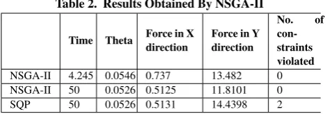
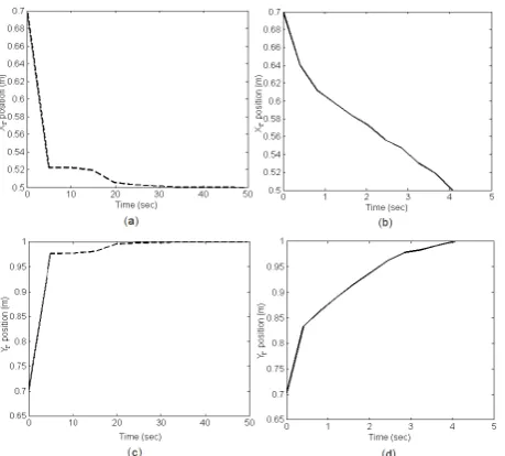
positioning payload, (ii) operational time and (iii) swing of pay-load. Fig 4, Fig 5 and Fig 6 shows the simulation result using NSGA-II and the results obtained indicates that our approach is a viable alternative. The NSGA-II algorithm was able to find minimum time without drastic increment in the forces required for positioning. The result obtained for minimum time and for maximum time required is presented in Table 2. For comparison
Table 2. Results Obtained By NSGA-II
Time Theta Force in X direction
Force in Y direction
No. of con-straints violated NSGA-II 4.245 0.0546 0.737 13.482 0 NSGA-II 50 0.0526 0.5125 11.8101 0
[image:6.595.314.553.700.782.2]purpose result obtained by SQP solver is given. SQP solver finds local optimal solution violating 2 strict constraints.
Fig. 4. (a) Load angle as function of time for maximum time (b) Load angle as function of time for minimum time
Fig. 5. (a) TheXrposition as a function of time for maximum
time (b) TheXrposition as a function of time for minimum time (c)
TheYrposition as a function of time for maximum time (d) TheYr
position as a function of time for minimum time
6. CONCLUSION
[image:7.595.57.285.135.249.2]This paper proposes a new approach to solve optimal control problems for mechanical systems. Discrete mechanics provides constraint equations and objective function while preserving the sympletic structure and the momentum maps corresponding to symmetry groups for the discrete solution. SQP (non-linear op-timization) method used to find local optimum to these equa-tions performs single objective optimization using initial guess. SQP method is applicable to smooth equations. This method can be replaced by an efficient global multi-objective optimization method, NSGA-II. The proposed approach is validated by find-ing optimal operatfind-ing conditions of 2D SpiderCrane, in carryfind-ing a load over a distance. Using the simulation results obtained by a single-objective SQP solver and multi-objective NSGA-II, we have shown that NSGA-II is a viable alternative to SQP solver.
Fig. 6. (a) Control force inXrdirection for maximum time (b)
Control force inXrdirection for minimum time (c) Control force in Yrdirection for maximum time (d) Control force inYrdirection for
minimum time
7. REFERENCES
[1] Kalyanmoy Deb,Multi-Objective Optimization Using Evo-lutionary Algorithms, Department of Mechanical Engineer-ing, Indian Institute of Technology, Kanpur, India. [2] Kalyanmoy Deb, Samir Agarwal, Amrit Pratap, T
Meyari-van,A Fast Elitist Non-Dominated Sorting Genetic Algo-rithm for Multi-Objective Optimization: NSGA-II, IEEE Transactions on Evolutionary Computation, 6(2):182 - 197, April 2002.
[3] Cadzow, J. A. , Discrete calculus of variations, Interna-tional Journal of Control 11, pages 393-407, 2010. [4] O. Junge and Sina Ober-Bl¨obaum,Optimal reconfiguration
of formation flying satellites, IEEE conference on Decision and Control and European Control Conference ECC, pages 66-71, Seville, Spain 2005.
[5] O. Junge, J. Marsden, and S. Ober-Bl¨obaum,Discrete me-chanics and optimal control,16thIFAC World Congress, pages 1-6, 2005.
[6] J. E. Marsden, M. West, Discrete Mechanics and Vari-aional Integrators, Acta Numerica (2001), pp. 1-158, Cam-bridge University Press, 1999.
[7] Bomze, I. M. and Di Pillo, Nonlinear optimization, Springer, 2010.
[8] D. Buccieri, Ph. Mullhaupt and D. Bonvin,Spidercrane: Model and Properties of a Fast Weight Handling Equip-ment,16thWorld Congress, The International Federation of Automatic Control, pages Th-A03-TO/2, July 2005. [9] Faruk Kazi, Ravi N. Banavar, Philippe Mullhaupt, and
Do-minique Bonvin,Stabilization of a 2D-SpiderCrane Mech-anism using Damping Assignment Passivity-based Control, Proceedings of the 17th World Congress The International Federation of Automatic Control Seoul, Korea, July 6 - 11, 2008
[10] I. Sarras, F. Kazi, R. Ortega, R. Banavar Total Energy-Shaping IDA-PBC Control of the 2D-Spider Crane,49th IEEE Conference on Decision and Control, pages 1122-1127, Dec 2010.
[image:7.595.56.286.328.535.2]ESAIM: Control, Optimisation and Calculus of Variations, pages 322-352, 2010.
[12] S. Ober-Blobaum,Discrete mechanics and optimal control, Ph.D. Thesis, University of Paderborn, Germany , 2008.
[13] Sushant Bahadure, C. Venkatesh, R. Mehra, F. Kazi, N. SinghStructure Preserving Optimal Control of 2D Spider-Crane, IEEE Systems Conference, Pages 585-589, March 2012.
[14] N. Srinivas and Kalyanmoy Deb,Multiobjective Optimiza-tion Using Nondominated Sorting in Genetic Algorithms, Evolutionary Computation, 2(3):221 - 248, 1994.
[15] A. K. Kamath, N. M. Singh, F. Kazi, R. Pasumarthy, Dy-namics and Control of 2D SpiderCrane: A Controlled La-grangian Approach, 49th IEEE Conference on Decision and Control, pages 3596-3601, Dec 2010.
[16] A. K. Kamath, N. M. Singh, F. Kazi,Dynamics and Control of 2D Spider- Crane: A RHC approachProceedings
Math-ematical Theory of Networks and Systems, pages 885-892 2010.
[17] G. Gogte, Venkatesh C., F.Kazi, N. M. Singh,Passivity Based Control Of Underactuated 2-D SpiderCrane Manip-ulator, MTNS, 2012.
[18] Kalyanmoy Deb, N. K. Gupta,In Search of Optimal Op-erating Principles for An Overhead Crane Maneuvering Using Multi-Objective Evolutionary Algorithms, KanGAL, Department of Mechanical Engineering, IIT Kanpur, Kan-GAL Report Number 2004011.
[19] R. Ortega, M. W. Spong, F. Gomez-Estern, G. Blankestin Stabilization of a Class of Underactuated Mechanical Sys-tems via Interconnection and Damping Assignment, IEEE Trans. Automat. Contr., vol. 47, Aug. 2002.