http://dx.doi.org/10.4236/am.2014.514210
Experiment Design for the
Location-Allocation Problem
María Beatríz Bernábe Loranca, Rogelio González Velázquez, Martín Estrada Analco,
Mario Bustillo Díaz, Gerardo Martínez Guzman, Abraham Sánchez López
Computer Science Department, Benemérita Universidad Autónoma de Puebla, Puebla, México Email: [email protected]
Received 10 June 2014; revised 11 July 2014; accepted 18 July 2014
Copyright © 2014 by authors and Scientific Research Publishing Inc.
This work is licensed under the Creative Commons Attribution International License (CC BY).
http://creativecommons.org/licenses/by/4.0/
Abstract
The allocation of facilities and customers is a key problem in the design of supply chains of com-panies. In this paper, this issue is approached by partitioning the territory in areas where the dis-tribution points are allocated. The demand is modelled through a set of continuous functions based on the population density of the geographic units of the territory. Because the partitioning problem is NP hard, it is necessary to use heuristic methods to obtain reliable solutions in terms of quality and response time. The Neighborhood Variable Search and Simulated Annealing heuristics have been selected for the study because of their proven efficiency in difficult combinatorial opti-mization problems. The execution time is the variable chosen for a factorial experimental design to determine the best-performing heuristics in the problem. In order to compare the quality of the solutions in the territorial partition, we have chosen the execution time as the common parameter to compare the two heuristics. At this point, we have developed a factorial statistical experimental design to select the best heuristic approaches to this problem. Thus, we generate a territorial par- tition with the best performing heuristics for this problem and proceed to the application of the location-allocation model, where the demand is modelled by a set of continuous functions based on the population density of the geographical units of the territory.
Keywords
Demand, Experimental Design, Heuristics, Location-Allocation, Partitioning.
1. Introduction
analysis to groups or zones under geographical aggregation using hierarchical grouping or partitioning methods fitting the problem.
For aggregation, this work uses as elements to be grouped the geographic territorial unit known as Basic Geo- Statistical Area (Ageb), defined as the minimum geographic division used for census and statistical purposes. The groups are comprised by a set of Agebs, considering within the grouping the properties of partitioning and the feature of compactness.
Solving geographical aggregation is a necessary task in territorial design problems and has been framed as a combinatorial problem of geographical partitioning or as geographical clustering [2] [3]. The aggregation being solved so far groups Agebs where the implicit objective function evaluates the minimum cost of the distance between them. This problem is discrete and mixed-integer; it has been formulated as a model of combinatorial optimization under the compactness criterion as an objective function where the associated partitioning algo-rithm is based on the classical partitioning algoalgo-rithms [4].
The combinatorial nature of Agebs partitioning involves the use of approximate methods [5], therefore in solving them, heuristic methods of confirmed efficiency when applied to difficult combinatorial problems have been used: Variable Neighborhood Search (VNS) and Simulated Annealing (SA) [2] [6].
With the goal of evaluating the quality of solutions from both heuristics and determining which one best ap-proximates the cost function for this problem; a statistical factorial surface response model has been used. Once the efficiency of VNS or SA has been guaranteed, the territory is partitioned in 8 groups to determine the distri-bution center for the location-allocation problem with dense demand. This Location-Allocation Problem (LAP) for a TDP with dense demand has the objective of finding the geographical coordinates (longitude, latitude) for the location of a Distribution Center (DC) that provides a service to a group of communities contained in each Ageb, which is represented by a centroid. The location of the DC must be the one which minimizes the travel expenses by finding the geographical center coordinates of all centroids. These community populations repre- sent potential clients for the DC and their demand is modeled by a continuous two-variable function based on the population density of each group [7].
An application of this approach is the location of medical health centers for each community at the centroid of each Ageb and the location of a general hospital at the geographical center of the centroids, which operates as a DC in such a way that a patient transfer requires minimal time. In geographical terms the terrestrial globe, after applying a suitable geographical projection, is considered as a subset of the cartesian plane. In the proposed me-thodology the solutions are taken as
( )
x y, points in R2 using geographical coordinates, where x is the longitude coordinate and y the latitude coordinate. Due to the numeric nature of the obtained solutions, the problem comprises a continuous case of the LAP. In addition to the mathematical formulation of the problem a Geographical Information System (GIS) is used with the purpose of creating maps via spatial data files and to perform information queries on the geographical zones [8].The structure of this paper is organized as follows: Introduction as Section 1; in Section 2 important aspects of territorial design are covered; the experiment designs methodology is described in Section 3. Section 4 presents a comparison between the response times of VNS and SA. In Section 5, we present our model and me-thodology for the Location-Allocation Problem. Finally, section 6 deals with the conclusion and future remarks.
2. Territorial Partitioning
In general, the problem of territorial design is defined as the collection of basic geographical units into large groups known as territories. An acceptable grouping is the one which fulfills certain predetermined criteria for a specific territorial design problem. These criteria can be economical, demographical, location-allocation of ser-vices, among others [1]. This work requires a territorial grouping, which involves the partitioning of the territory under study. The partitioning of the territory has been the result of implementing an algorithm where the crea-tion of groups is performed based on the property of geometric compactness of territorial design and the mini-mization of distances between centroids [2].
2.1. Formulation of the Territorial Partitioning Problem
{
1, 2, , j, , n}
T = A A A A such that
1 n
j j
T =
= A and Ai∩
Aj =∅ ∀ ≠i j and let C={
c c1, 2,,cj,,cn}
be the set of centroids of each Ageb in T, where cj=
(
x xi, j)
. We want to form a set P, 1< <p n,{
1, 2, , k, , n}
P= G G G G such that P is a partition of T and each Gk is a collection of Agebs. Under the criterion of geographical compactness the objective function to be minimized consist of the Euclidean distance from one of the p centroids cj to every other centroid ci of the same group Gi and the solution space Ω is the set of all partitions of T with cardinality p:
(
)
Ω 2
min , 1,2, ,
i k
n
j c G j i
P∈
∑ ∑
= ∈ d c c ∀ =k p(1)
Equation (1) corresponds to the objective function of the partitioning problem. Note that in the case of a search by exhaustive enumeration in Ω the number of alternative solutions that must be examined to find the solution is given by
(
!)
Ω! !
n n
p p n p
= = −
(2)
where n is the number of Agebs and p is the desired number of groups.
While Equation (2) suggests that the complexity order is O n
( )
p for pn and consequently polynomial in n for a given value of p, the number of combinations is quite large [9].( )
1 2 1 2
n n n
p n O p = = − =
∑
(3)For variable values of p the problem are still NP-complete since the time required to solve by exhaustive search grows exponentially in n this justifies the use of a metaheuristic) [5].
To manage the computational cost, VNS and SA have been implemented. This section examines VNS in de-tail due to the fact that in the exercise of the statistical experiment, it was proven that VNS responds with better solutions for the territorial partitioning problem exposed in this work (this reason justifies the use of VNS as ap-proximation method).
2.2. Basic Variable Neighborhood Search
The Variable Neighborhood Search (VNS) meta-heuristic has been incorporated to the territorial partitioning problem to obtain approximate solutions. We have abstracted the essential aspects of VNS and Variable Neigh-borhood Search Descendent (VNSD) to simplify them into a single flexible and easy algorithm to be used in several implementations for partitioning problems as is shown in the following procedure [10] [11]:
Procedure 1. VNS.
Require Number of Structures NS, Local Search LS and Input Instance. 1) Nk ← Neighborhood Structures k th− , k=1, 2,,NS;
2) Generation (Initial Solution); 3) For k=1 to NS do;
4) Current Solution ← Local Search
k
N (Initial solution);
5) Initial solution ← Current Solution; 6) End for;
7) Best Solution ← Initial solution; 8) ReturnBest Solution.
The parameters in this procedure include Neighborhood Structures (NS) and Local Search (LS), which are considered to be evaluated by the statistical experiment. It is convenient to review the way that the neighbor-hoods are generated in VNS from an initial solution. This implementation can be seen in [2].
3. Experiment Designs to Determine the Parameters in the Metaheuristics
3.1. Response Surfaces
The Response Surface Methodology (RSM) is a collection of techniques that allow inspecting a response that can be represented by a surface, when the experiments explore the effect of the variation of quantitative factors in the values of a dependent variable or response variable [12]. This methodology tries to find the optimal values for the independent variables to maximize, to minimize or just to meet some constraints in the response variable. The trend in the development of RSM has been the construction of compact designs of experiments, with a minimum of experimental designs. Thus the researcher focuses in the properties of the estimators of all the pa-rameters of the response function, which depend on the type of design used.
To estimate a response surface, the linear models of order less than or equal to three have been employed fre-quently because of their simplicity and easy interpretation. However, [13] show that the fractional polynomials can make a better approximation in some experiments. The bases of the RSM are obtained from the theory of the general linear model. It is assumed that the response variable depends on the independent variables through a function f that can be complex or unknown. The function is approximated in the region of interest by a poly-nomial of low order, generally less than or equal to three, or pseudo-quadratic. To evaluate the efficiency of the estimators of a response surface several procedures have been proposed based on the bias. This is the case of the mean square error (MSE) that also has been taken as a base to obtain others like that proposed by [14]. There are several classes of designs developed for the approximation of a surface of second order that require less combi-nations of treatments than the factorial designs, with different characteristics and properties. Among these, the central composite designs proposed by [12] do not grow as fast as the factorial designs or the Box-Behnken de-signs.
3.2. Central Composite Design
We use central composite designs to study the Variable Neighborhood Search metaheuristic. The factors are co-dified since it is easier to work with the levels of coco-dified factors in a uniform framework to analyze the effects of the factors. The levels of the codified factors in a 2k
factorial design are
(
i)
i
A A X
D − =
where Ai is the ith level of the factor A, A is the average level of factor A and D=1 2
(
A3−A1)
[15]. The central composite designs are designs of 2k factorial treatments with 2k additional combinations called axial points and nc center points. The coordinates of the axial points of the axes of the codified factor are(
±α, 0, 0,, 0 , 0,) (
±α, 0, 0,, 0 ,)
, 0, 0,(
,±α)
and the center points have the form(
0, 0,, 0)
. De-pending on the election of α in the axial points, the central composite design has different properties such as orthogonality, rotatability and uniformity. We will consider only one desirable property in these designs that re-quires the variance of the estimated values to be a constant in equidistant points from the center of the design.This property is called rotatability, and is achieved making α =
( )
2k 1 4. In this way, the value of α or design with two factors isα
=1.414 and for three factorsα
=1.682. The formula for α changes if replicates of the design are done or if a fractional factorial design is used [16].3.3. Determination of VNS and SA Parameters for the Territorial Partitioning Problem
In this section, the statistical procedure that has been followed to get adequate parameters for the heuristics to compare is exposed. For VNS the application of a central composite design is proposed and for SA a Box Behnken. Finally, the needed tests are done to model the parameters and finding adjusted times in order to be able to compare the two heuristics in an unbiased way when the time (T, seconds) has been chosen as a colleting parameter.VNS Parameters for the Territorial Partitioning Problem under a Central Composite Design
meters ensures their usefulness in this work.
We have started with the study over a set of tests to prove the general functionality: the response time must considerably reduce the computational cost and the quality of the solutions must be very close to the optimal. Due to the fact that we are interested in adjusting the VNS parameters to set the time as the comparison factor with SA, in this first experiment the cost function is just the time (T, seconds).
Previous studies have been revised to build diverse experiments with the goal of finding strategic values for the proposal of an experimental design that provides the balance of competitive parameters for VNS [2].
A composite central design was used with a high level of 1718 and 1365 as the low level for neighborhood structures (NS). In Local Search (LS) 1031 has been determined as the low level and 1370 as the high level.
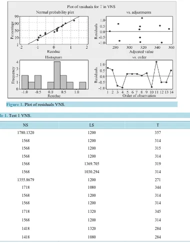
[image:5.595.114.494.239.723.2]The associated experiment can be seen in the next Table 1 and Figure 1attached indicates that the data be-haves normally, that the second order model is adequate and that there’s no effect between runs in the experi- ment. The regression model of second order exits statistical evidence for the reliability of the experiment:
[image:5.595.129.468.241.442.2]Figure 1. Plot of residuals VNS.
Table 1.Test 1 VNS.
NS LS T
1780.1320 1200 357
1568 1200 314
1568 1200 315
1568 1200 314
1568 1369.705 319
1568 1030.294 314
1355.8679 1200 271
1718 1080 344
1568 1200 314
1568 1200 314
1718 1320 345
1568 1200 314
1418 1320 284
3.4. Simulated Annealing Parameters Determination for the Territorial Partitioning
Problem with Box Behnken
The Box Behnken (BB) design is an independent quadratic design that doesn’t possess a factorial or a fractional factorial design. These designs are revolving (or almost revolving) but they possess limited capacity of ortho-gonal blocking compared with the Central Composite Design (CCD).
The Box Behnken Design for 3 factors involves 3 blocks, in each one of them 2 factors are varied through the 4 possible high and low combinations. Is furthermore necessary to include central points, where all of the factors are in their central values. In consequence, these designs don’t contain points in the vertex of the experimental region. The number of experiments required
( )
N is defined by the expression(
)
2 1
N= k k− +Co
where k is the number of factors and Co is the number of central points [16].
Simulated Annealing
Simulated Annealing (SA) is a neighborhood search algorithm with probabilistic criteria to accept solutions based on thermodynamics, is a neighborhood search method characterized by a neighboring solutions accep- tance criterion that adapts along its execution. In general, SA is a metaheuristic which combines the principles of the basic local search and the probabilistic Monte Carlo approach [6].
The temperature
( )
t is important in SA and determines in what measure worse neighboring solutions than the current can be accepted. The variable t is initialized with a high value, denominated initial temperature( )
TI and is reduced in every iteration by means of a cooling mechanism𝛼𝛼(alpha), until a final temperature( )
TF is reached. In each iteration a concrete number of neighbors, L t( )
is generated that can be fixed for all of the execution or depend on the concrete iteration [6]. In this work L t( )
has been denoted by LT.We are betting on determining values in the SA parameters so they can be compared in a fair way with VNS, being the time
( )
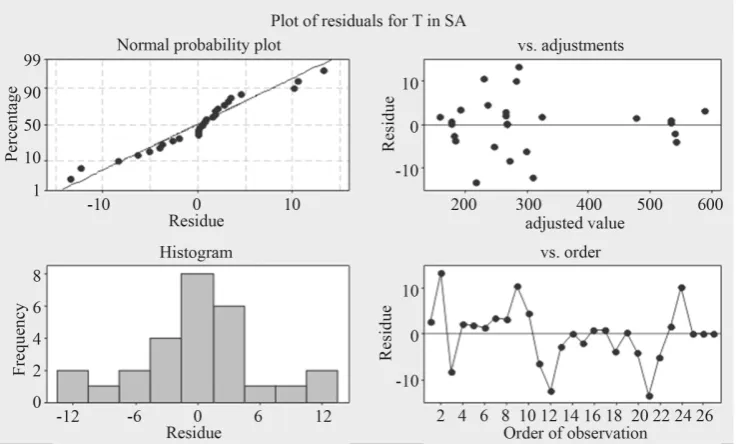
T of execution the common parameter for the 2 heuristics under study. To get close to convenient parameters, the first part of the tests was experimental and random. Considering the times obtained in the Table 1 for VNS, diverse instances were created for SA relying on their respective BB (to trust in the suitability of the model). The next design was achieved and its model and instances can be seen in the Table 2 [image:6.595.115.484.482.706.2]and the Figure 2 shows that the data behaves normally and that there’s no effect between runs in the experi- ment:
Table 2. Experiment for SA.
TI TF α LT T
81,000 0.09 0.98 3000 267
99,000 0.09 0.98 3000 300
81,000 0.11 0.98 3000 264
99,000 0.11 0.98 3000 268
90,000 0.1 0.97 2700 160
90,000 0.1 0.99 2700 480
90,000 0.1 0.97 3300 195
90,000 0.1 0.99 3300 592
81,000 0.1 0.98 2700 239
99,000 0.1 0.98 2700 240
81,000 0.1 0.98 3300 293
99,000 0.1 0.98 3300 296
90,000 0.09 0.97 3000 179
90,000 0.11 0.97 3000 177
90,000 0.09 0.99 3000 540
90,000 0.11 0.99 3000 535
81,000 0.1 0.97 3000 178
99,000 0.1 0.97 3000 180
81,000 0.1 0.99 3000 535
99,000 0.1 0.99 3000 540
90,000 0.09 0.98 2700 203
90,000 0.11 0.98 2700 240
90,000 0.09 0.98 3300 325
90,000 0.11 0.98 3300 292
90,000 0.1 0.98 3000 268
90,000 0.1 0.98 3000 268
90,000 0.1 0.98 3000 268
4. Modeling of the Response Times for VNS and SA in Instances of 8 Groups
Reviewing Section 3 and after having carried out the corresponding runs for SA and VNS, it is necessary to model the associated parameters to calibrate them in such a way that is possible to optimize the response time, which will be in function of the values of the parameters.
4.1. Modeling of the Response Times for VNS
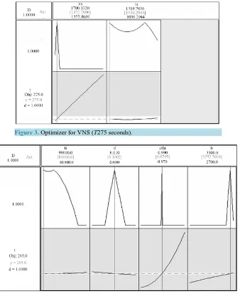
tween 280 and 340 seconds while the values for Local Search (LS) are between 1050 and 1350 iterations, and Neighborhood Structures (NS) bounded by 1400 and 1750 iterations. With this values it has been possible reach the compromise now is to get the exact parameters to run VNS in the established times, then, under the model of second order, graphs were obtained that reflect the measure of the parameters to obtain the Cost Function (CF), that in this case is the time. The optimization graphs are presented for the cases of 275 seconds (see Figure 3, where NS=ns, LS=ls and T =t).
4.2. Modeling of the Response Times for SA in Instances of 8 Groups
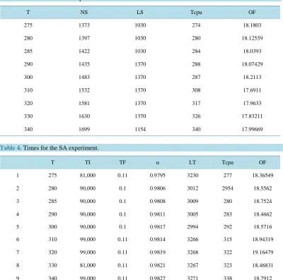
From the results achieved for SA (see Table 2), diverse contour graphs were done. A contour graph was picked, that as well as VNS, shows distinct units of times
( )
T estimated in seconds: 275, 285, 290, 300, 310, 320, 330 and 340 and the parameters of alfa and LT are fixed at 0.98 and 3000 units respectively. TF is between 0.90 and 0.110 while TI oscillates in 8200 and 9800 units (iterations). Relying on all of the results obtained until now and with the model of second order, is possible to create a model to find a balance of the SA parame-ters and to reach a cost for the selected times. In the graphic of optimization showed in Figure 4, the calibration of the parameters can be seen to obtain a cost function of 285 seconds. The notation in this Figure 4 is TI=ti, [image:8.595.133.471.293.709.2]TF=tf , LT=lt, and T =t.
Figure 3. Optimizer for VNS (T275 seconds).
4.3. Response Times Comparison
The challenge at this point is to check that VNS and SA execute within the time we have found where both heu-ristics must run in the same time when the parameters have indicated the time in which they must execute for determined values. The next step consist in doing the associated tests and verifying that with calibration of the parameters for SA and VNS they achieve a cost function in a determined time, in this way we can observe which heuristic offers better quality in the solutions.
In Table 3, the values of the Objective Function (OF) and the cpu time (T cpu) have been recorded for the parameters of VNS suggested by the statistical model that has been developed. It is clear to note that the real computing times (T cpu) are almost “exact” with the ones estimated by the model.
In a similar form, in Table 4 the values of the objective function and the T cpu time have been ordered for the parameters of SA given by the statistical model that has been developed. The real computing times are much approximated with the ones estimated by the model.
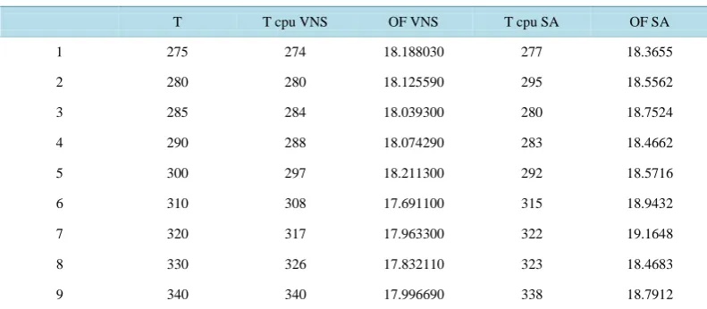
Finally, the results of the times and objective function for SA and VNS were gathered. In Table 5, it can be observed that VNS reaches better values of the cost function in instances of 8 groups.
Having obtained these results, our interest now is to solve the aspect of the dense demand.
The best cost of the OF for VNS has been chosen and to initiate the study with parameters of neighborhood structure NS=1532 and local search LS=1370.
Table 3. Times for the VNS experiment.
T NS LS Tcpu OF
275 1373 1030 274 18.1803
280 1397 1030 280 18.12559
285 1422 1030 284 18.0393
290 1435 1370 288 18.07429
300 1483 1370 287 18.2113
310 1532 1370 308 17.6911
320 1581 1370 317 17.9633
330 1630 1370 326 17.83211
[image:9.595.99.500.315.712.2]340 1699 1154 340 17.99669
Table 4.Times for the SA experiment.
T TI TF α LT Tcpu OF
1 275 81,000 0.11 0.9795 3230 277 18.36549
2 280 90,000 0.1 0.9806 3012 2954 18.5562
3 285 90,000 0.1 0.9808 3009 280 18.7524
4 290 90,000 0.1 0.9811 3005 283 18.4662
5 300 90,000 0.1 0.9817 2994 292 18.5716
6 310 99,000 0.11 0.9814 3266 315 18.94319
7 320 99,000 0.11 0.9819 3268 322 19.16479
8 330 81,000 0.11 0.9821 3267 323 18.46831
Table 5. Times and OF for SA and VNS.
T T cpu VNS OF VNS T cpu SA OF SA
1 275 274 18.188030 277 18.3655
2 280 280 18.125590 295 18.5562
3 285 284 18.039300 280 18.7524
4 290 288 18.074290 283 18.4662
5 300 297 18.211300 292 18.5716
6 310 308 17.691100 315 18.9432
7 320 317 17.963300 322 19.1648
8 330 326 17.832110 323 18.4683
9 340 340 17.996690 338 18.7912
5. Model and Methodology for Location Allocation Problem
This section describes the mathematical model and the basic methodology to solve the location-allocation prob-lem for a territorial design probprob-lem with dense demand.
The Location-Allocation Problem will be denoted as LAP. The LAP is an optimization problem, classic in the location theory that is often used in territorial design problems TDP. With the Agebs well defined when solving it, the location of the facilities is determined and the clients are allocated to each facility. The territorial design problem can be studied by means of the P-Median Problem that we'll denote as PMP. The location-allocation problem belongs to the problems class NP-complete [5]. The problem solved in this work gives answer to the problem of locating facilities and allocating clients in dense demand scenarios in TDP. The computing complex-ity of PMP makes necessary the appliance of a metaheuristic as approximation procedure to the optimal solu-tion.
The development of the proposal of the p-median problem had place in the 60’s and the direct case can be at-tributed to Hakimi and to Weber, the continuous case [9] [17]. The p-median consists of a given set of n ver-tices and a distances (or costs) matrix between the verver-tices, p vertices must be chosen with the purpose to mi-nimize the sum of the distances of all the points to the closest chosen selected point. In 1970, the first integer programming formulation for the p-median problem is presented, cited in [17]. In general, the P-Median Prob-lem can be mathematically expressed as a discrete optimization probProb-lem. First we denote the distances matrix as
ij
d that expresses the distance between the potential location points i and the demand points j. Two binary variables are introduced, the first one xij corresponds to the location of the demand point j to the facility i or not and the second yi indicates that a facility is established in the point i or not, and can be proposed as a binary integer problem in the following way:
Let
1 if the point is assigned to point
0 otherwise
ij
j i
x = and
1 if a facility is located in point 0 otherwise
i
i y =
1 1
minZ =
∑ ∑
ik= nj=d xij ij (4)Subject to
1 1 1, 2, , ;
k ij
i= x = ∀j= n
∑
(5)1 1, 2, , ;
n
ij i
j= x ≤ny ∀ =i k
1
n i j= y = p
∑
(7) where dij is the distance between the centroid j and the Ageb i and k is the number of potential vertices where a median can be located, generally k=n p, is the fixed number of required medians. Equation (4) is the objective function that minimizes the system’s distance, the restriction 5 establishes that each demand point can only be allocated to one facility. The restriction 6 establishes the allocation of demand points to each of the fa-cilities or medians and finally the restriction 7 guarantees that among the k potential location points exactlyp are chosen.
Given a set of customers spread over a territory 2
R
⊆ , P=
{
G G1, 2,,Gp}
a partition of T in p groups,each Gi =
{
A A1, 2,,Aj}
∈P , ∀ =i 1, 2,,p and j=1, 2,,Gi a partition of each element of P inAgebs. Each Aj has a representative called centroid Ageb denoted by ci =
(
x yi, i)
obtained by the formulas (11) from which each community is served. Each point p x y( )
, ∈Gi, has a density of demand given by( )
(
,)
D p =D x y . Let d p c
(
, i)
be the Euclidean distance from any point p to the centroid. The cost of transportation from a point p to the centroid ci is defined as D p d p c( ) (
, i)
.The solution consists in finding the coordinates from a point
(
x y,)
∈Gi such that the cost of the transporta- tion is minimized from each community to a central facility. The conditions to be satisfied by forming joint par- titions of T and of Gi are that they are disjoint, namely Gi∩
Gr =∅ and Aj∩
As =∅ , ∀ ≠i r and j≠s. The mathematical model that represents the mentioned conditions is the following:( )
(
)
(
) (
)
2 2 2 , min , i n j j jx y∈GTC=
∑
= D x y x−x + y−y (8)Subject to
2
p i i= G =T
(9)1 1, 2, , ;
i
G
i i
j= A =G ∀ =i p
(10)The objective function TC represented in Equation (8) is the total cost of transportation, and Equations (9) and (10), are the constraints of the partitioning of the territory T and the Gi. But in practice we define the in-stances under the general PMP definition as POC and also its instance as follows:
Given a set =
{
1, 2,,m}
of 𝑚𝑚 potential facilities and a set U={
1, 2,,n}
of n users, a matrix( )
ij n mD= d ×
where dij represents the euclidean distance between users ui and the facilities fj, ∀ ∈i U j, ∈, a prede-fined p<m, then an instance of PMP is denoted by PMP
(
, , ,U D p)
.A feasible solution for PMP
(
, , ,U D p)
is a subset J⊂, J = p, which cost function is defined by(
, , ,)
minJ ij
j J i U
C U D p d
∈ ∈ =
∑
.
The objective of PMP is to find a feasible solution J* such that
(
)
(
{
(
)
}
)
* , , , min j , , , Ω
J
C U D p = C U D p J∈
where Ω is the set of all the feasible solutions.
The PMP consists in determining simultaneously the positions of in which the p services must be lo-cated, in such a way that the total transport cost necessary to satisfy the demands of the users is minimized, supposing that said cost is proportional to the amount of demand and the traveled distance. For that, each user will be attended by the closest plant or service.
The sequence of necessary steps to obtain the coordinates of the central facility in a cluster is as follows: Define the parameters for the partitioning of the territory T.
Generate the partitioning with the VNS metaheuristic.
With the file obtained from step 2, generate a map within a map using a GIS.
Calculate the centroids of each AGEB, using calculus Formulas (11). Apply the Equation (8) to the chosen cluster.
( )
( )
( )
( )
, d d , d d
and
, d d , d d
i i
xp x y x y yp x y x y
x y
p x y x y p x y x y
=
∫∫
=∫∫
∫∫
∫∫
(11)Equations (11) are the classical calculus formulas used to calculate the centroid of a metallic plate with den-sity
ρ
[18]. In this paper, we consider the Agebs as if they were metallic plates with population density given by ρ(
x y,)
.5.1. Response Surfaces
In this subsection, the proposed methodology has been implemented for the Metropolitan Zone Toluca Valley (MZTV).
Having partitioned the territory in 8 groups, we select one of the clusters to apply the experiment and this consists of obtaining the centroid for each Ageb, and then calculating the center of the centroids. Finally, the re-sults of the implementation are shown.
Implementation of the Methodology to the Metropolitan Zone Toluca Valley
For the implementation, is necessary to have the data that describes the MZTV as a geographical area, as well as to have a geographical partition that represents the particular problem. The partition of the MZTV consists of the formation of five clusters of Agebs, according to the criteria of compactness of the clusters. The method in this section has been characterized as TDP. Furthermore, it is a COP classified as NP-complete and is therefore ad-visable to apply a metaheuristic, as we mentioned in Section 2. Basically, the sequential strategy to resolve the case study in this paper is to follow six steps.
1) The partition parameters are defined. The input to the VNS program is a file that contains the geographical data of the MZTV. The number of clusters to be formed, the number of VNS iterations, and the number of itera-tions of the local search are introduced.
2) The VNS program is run to obtain a file that contains the Agebs of each of the clusters that make up the MZTV, as well as the run time and the cost associated with the partition.
3) With the exit file of step 2, a map is generated. The map contains the partition corresponding to the running of the VNS program for the MZVT.
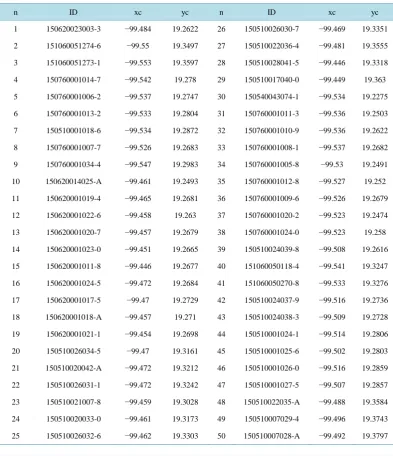
4) A cluster of the partition is selected. For our case study, we select one cluster. The Ageb codes are in the first column of Table 6. We associate a density of demand function to this cluster. This function is taken one at a time from the set of six linear functions, and two non-linear ones from Table 7, denoted by LD1, LD2, LD3, LD4, LD5, LD6 y NLD1, NLD2 respectively, and proposed by Murat [19].
5) The file, with the codes of the Agebs of the MZTV is introduced into a GIS to obtain a map. 6) Finally, the coordinates for the center of the centroids are obtained by applying the model.
Table 6 shows the results that were obtained from the sequential program designed for VNS on the graphical data of the MZTV for each density of demand function associated with the Agebs. To obtain the geo-graphical coordinates of the center of the centroids, a non-linear programming problem was resolved using the optimization tool Solver Excel.
Table 8 shows the results of eight different density functions, arranged in rows and columns in the following way: the first column corresponds to the objective function Z, that is defined as the product of the function of density of demand, multiplied by the distance from the point p to each centroid ci, in the second and third columns are the decimal coordinates of the center of the centroids. The objective functions used in this work are convex functions.
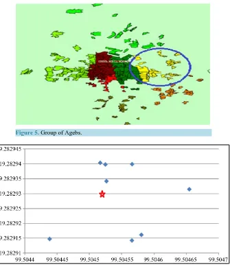
Figure 5 is the selected group under study (blue circle).
The results in columns 3 and 4 in Table 8 show the coordinates of eight possible points to locate the center of centroids. These points are associated to different functions of demand density for the MZTV instance. Figure 6
Table 6.Key Agebs and coordinates of centroids.
n ID xc yc n ID xc yc
1 150620023003-3 −99.484 19.2622 26 150510026030-7 −99.469 19.3351
2 151060051274-6 −99.55 19.3497 27 150510022036-4 −99.481 19.3555
3 151060051273-1 −99.553 19.3597 28 150510028041-5 −99.446 19.3318
4 150760001014-7 −99.542 19.278 29 150510017040-0 −99.449 19.363
5 150760001006-2 −99.537 19.2747 30 150540043074-1 −99.534 19.2275
6 150760001013-2 −99.533 19.2804 31 150760001011-3 −99.536 19.2503
7 150510001018-6 −99.534 19.2872 32 150760001010-9 −99.536 19.2622
8 150760001007-7 −99.526 19.2683 33 150760001008-1 −99.537 19.2682
9 150760001034-4 −99.547 19.2983 34 150760001005-8 −99.53 19.2491
10 150620014025-A −99.461 19.2493 35 150760001012-8 −99.527 19.252
11 150620001019-4 −99.465 19.2681 36 150760001009-6 −99.526 19.2679
12 150620001022-6 −99.458 19.263 37 150760001020-2 −99.523 19.2474
13 150620001020-7 −99.457 19.2679 38 150760001024-0 −99.523 19.258
14 150620001023-0 −99.451 19.2665 39 150510024039-8 −99.508 19.2616
15 150620001011-8 −99.446 19.2677 40 151060050118-4 −99.541 19.3247
16 150620001024-5 −99.472 19.2684 41 151060050270-8 −99.533 19.3276
17 150620001017-5 −99.47 19.2729 42 150510024037-9 −99.516 19.2736
18 150620001018-A −99.457 19.271 43 150510024038-3 −99.509 19.2728
19 150620001021-1 −99.454 19.2698 44 150510001024-1 −99.514 19.2806
20 150510026034-5 −99.47 19.3161 45 150510001025-6 −99.502 19.2803
21 150510020042-A −99.472 19.3212 46 150510001026-0 −99.516 19.2859
22 150510026031-1 −99.472 19.3242 47 150510001027-5 −99.507 19.2857
23 150510021007-8 −99.459 19.3028 48 150510022035-A −99.488 19.3584
24 150510020033-0 −99.461 19.3173 49 150510007029-4 −99.496 19.3743
25 150510026032-6 −99.462 19.3303 50 150510007028-A −99.492 19.3797
Table 7.Set of density of demand functions.
D(x, y)
LD1 7.5x + 7.5y + 100
LD2 10x + 5y + 100
LD3 (100/7)x + (5/7)y + 100
LD4 (10/3)x + (5/3)y + 600
LD5 2.5x + 2.5y + 600
LD6 (100/21)x + (5/21)y + 600
NLD1 (9/80)x2 + (9/80)y2 + 100
[image:13.595.98.487.573.717.2]Figure 5.Group of Agebs.
[image:14.595.102.496.498.663.2]Figure 6.Location of nine points, where eight of them belong to the coordinates in Table 8.
Table 8.Times and OF for SA and VNS.
Z x_c y_c
Z × LD1 1864.0328 −99.5045168 19.2829403
Z × LD2 1170.8971 −99.5045248 19.2829398
Z × LD3 3052.2653 −99.5045265 19.2829342
Z × LD4 701.2759 −99.5045804 19.2829162
Z × LD5 932.3211 −99.5045658 19.2829143
Z × LD6 305.1979 −99.5046545 19.2829315
Z × NLD7 2930.8736 −99.5045169 19.2829294
Z × NLD8 4529.6747 −99.5044387 19.2829148
point, is calculated as the point with minimal distance to the other eight points and we may name it as the center of centers.
the location of the center may be any point into the circle defined by
(
) (
2)
2 2cc cc
x−x + y−y =r
where r=max
{
d P c(
c, j)
j=1, 2, 3,,8}
.6. Conclusion
The proposal in this work is a structure to solve location-allocation models based on Geographic Information Systems. The application is shown in the case study of the MZTV map. The methodology was tested in demand regions with irregular forms in comparison with previous works where regions are rectangular or convex poly-gons. Since the territory design problem is a hard combinatorial optimization problem, the use of metaheuristics allows obtaining a solution in areas or large size and partitions of high cardinality. According to the analysis of the results obtained, the integration of territorial design aspects with density functions in location-allocation models creates a wider range of possible applications to real problems, for example in supply chain design among others. Therefore, an important contribution of this work is the successful combination of three relevant aspects in real problems: territorial design, location-allocation decisions, and demand density functions. The as-sembly of several tools like metaheuristics, information systems and mathematical models provides a robust de-vice for application in visual environments, like maps, for the analysis of geo-statistical information.
References
[1] Zoltners, A.A. and Sinha, P. (1983) Towards a Unified Territory Alignment: A Review and Model. Management Science, 29, 1237-1256. http://dx.doi.org/10.1287/mnsc.29.11.1237
[2] Bernábe, M.B., Espinosa, J.E., Ramírez, J. and Osorio, M.A. (2011) A Statistical Comparative Analysis of Simulated Annealing and Variable Neighborhood Search for the Geographical Clustering Problem. Computación y Sistemas, 14, 295-308.
[3] Koskosidis, Y.A. and Powell, W.B. (1992) Clustering Algorithms for Consolidations of Customers Order in to Vehicle Ship Shipment. Transportations Research, 26, 325-379.
[4] Piza, E., Murilo, A. and Trejos, J. (1999) Nuevas Técnicas de Particionamiento en Clasficación Automática. Revista de Matemáticas Teoría y Aplicaciones, 6, 51-66.
[5] Altman, M. (1997) Is Automation the Answer: The Computational Complexity of Automated Redistricting? Rutgers Computer and Law Technology Journal, 23, 81-142.
[6] Kirkpatrick, S., Gelatt, C.D. and Vecchi, M.P. (1983) Optimization by Simulated Annealing. Science, 220, 671-680. http://dx.doi.org/10.1126/science.220.4598.671
[7] Newling, B.E. (1969) The Spatial Variation of Urban Population Densities. Geographical Review, 59, 242-252. http://dx.doi.org/10.2307/213456
[8] Zamora, E. (1996) Implementación de un Algoritmo Compacto y Homogéneo para la Clasificación de Zonas Geográficas AGEBs Bajo una Interfaz Gráfica. Thesis, Benemérita Universidad Autónoma de Puebla, México.
[9] Daskin, M.S. (1995) Network and Discrete Location, Models, Algorithms, and Applications. John Willey & Sons Ltd., Hoboken. http://dx.doi.org/10.1002/9781118032343
[10] Mladenovic, N. and Hansen, P. (1997) Variable Neighborhood Search. Computer Operation Research, 24, 1097-1100. http://dx.doi.org/10.1016/S0305-0548(97)00031-2
[11] Hansen, P., Mladenovic, N. and Moreno, P.J. (2010) A Variable Neighborhood Search: Methods and Applications.
Annals of Operations Research, 175, 367-407. http://dx.doi.org/10.1007/s10479-009-0657-6
[12] Box, G.E. and Wilson, K.G. (1951) On the Experimental Attainment of Optimum Conditions. Journal of the Royal Statistical Society, 13, 1-45.
[13] Cady, F.B and Laird, R.J. (1973) Treatment Design for Fertilizer Use Experimentation. CIMMYT Research Bulletin, 26, 29-30.
[14] Box, G.E. and Draper, NR. (1959) A Basis for the Selection of a Response Surface Design. Journal of the American Statistical Association, 54, 622-654. http://dx.doi.org/10.1080/01621459.1959.10501525
[15] Briones, E.F and Martínez, G.A. (2002) Eficiencia de Algunos Diseños Experimentales en la Estimación de una Super- ficie de Respuesta. Agrociencia, 36, 201-210.
[17] Church, R.L. (2003) COBRA: A New Formulation of the Classic P-median Location Problem. Annals of Operations Research, 122, 103-120. http://dx.doi.org/10.1023/A:1026142406234
[18] Bennett, C.D. and Mirakhor, A. (1974) Optimal Facility Location with Respect to Several Regions. Journal of Regional Science, 14, 131-136. http://dx.doi.org/10.1111/j.1467-9787.1974.tb00435.x
[19] Murat, A., Verter, V. and Laporte, G. (2010). A Continuous Analysis Framework for the Solution of Location—Allo- cation Problem with Dense Demand. Compute rs& Operations Research, 37, 123-136.
currently publishing more than 200 open access, online, peer-reviewed journals covering a wide range of academic disciplines. SCIRP serves the worldwide academic communities and contributes to the progress and application of science with its publication.
Other selected journals from SCIRP are listed as below. Submit your manuscript to us via either