Munich Personal RePEc Archive
Crash Risk Reduction at Signalized
Intersections Using Longitudinal Data
Burkey, Mark L. and Obeng, Kofi
North Carolina AT State University
2005
Online at
https://mpra.ub.uni-muenchen.de/36281/
Crash Risk Reduction at Signalized Intersections
Using Longitudinal Data
Mark L. Burkey, Ph.D.
Kofi Obeng, Ph.D.
Co-Principal InvestigatorsUrban Transit Institute
Transportation Institute
North Carolina Agricultural & Technical State University
B402 Craig Hall 1601 East Market Street
Greensboro, NC 27411
Telephone: (336) 334-7745 Fax: (336) 334-7093 Internet Home Page: http://www.ncat.edu/~traninst
Prepared for:
U.S. Department of Transportation Research and Special Programs Administration
Washington, DC 20590
DISCLAIMER
The contents of this report reflect the views of the authors who are responsible for the facts and the
accuracy of the information presented herein. This document is distributed under the sponsorship of the
Department of Transportation, University Research Institute Program, in the interest of information
1. Report No.
DTRS93-G-0018
2. Government Accession No. 3. Recipient’s Catalog No.
5. Report DateDecember 2004 4. TITLE AND SUBTITLE
CRASH RISK REDUCTION AT SIGNALIZED INTERSECTIONS USING
LONGITUDINAL DATA 6. Performing Organization Code
7. Author(s) MARK L. BURKEY, PH.D., KOFI OBENG, PH.D. 8. Performing Organization Report No. 10. Work Unit No.
9. Performing Organization Name and Address Urban Transit Institute The Transportation Institute NC A&T State University Greensboro, NC 27411
11. Contract or Grant No. DTRS93-G-0018
13. Type of Report and Period Covered
Final January 2004-December 2004 12. Sponsoring Agency Name and Address
US Department of Transportation
Research and Special Programs Administration 400 7th Street, SW
Washington, DC 20590 14. Sponsoring Agency Code
15. Supplementary Notes
16. Abstract
This study extends the previous work of Burkey and Obeng (2004) that examined the impact of red light cameras on the type and severity of crashes at signalized intersections in Greensboro, NC. The extension takes the following form. First, we extend the data to cover 57 months, and to include demographics, technology variables, the condition of a driver at the time of the crash, vehicle characteristics, land use and visual obstruction. Second, instead of examining the impact of red light cameras, we focus on identifying the
determinants of crash severity, two-vehicle crashes, and property damage costs. The major findings are that the safety impacts of seatbelt use outweigh the impacts of airbags deploying because the latter tends to increase evident injuries and property damage costs, while the former reduces these injuries. We also find that head-on collisions and under rides increase evident injuries. For two-vehicle crashes, we find that the risk of severe injuries increases in pickup-pickup crashes and SUV-pickup crashes, while the risk of possible injuries increases in car-truck crashes. For property damage costs, we found the condition of the driver at the time of the crash (i.e., illness, impaired, medical condition, driver falling asleep, driver apparently normal) to be important determinants in increasing these costs. The types of accidents that we found to increase property damage costs are running into a fixed object and under rides. Finally, we found that property damage costs of crashes are low where the land uses are commercial and institutional suggesting that the accidents that occur in these areas are minor.
17. Key Words
Longitudinal Data Accidents
Intersections
18. Distribution Statement
19. Security Classif. (of this report) UNCLASSIFIED
20. Security Classif. (of this page) UNCLASSIFIED
21. No. of Pages 48
TABLE OF CONTENTS
Executive Summary ... 1
Introduction ... 2
Literature Review... 3
Data... 7
Analysis of Crash-Level Severity ... 13
Determinants of Injuries in Two-Vehicle Crashes... 23
Land Use and Visibility Effects and Accident Rates ... 30
Determinants of Property Damage Costs ... 33
Conclusion... 40
References ... 44
Appendix ... 48
LIST OF TABLES 1. Comprehensive Costs of Crashes ... 5
2. Descriptive Statistics... 11
3. Binomial Probit: Fatality and Incapacitating Injuries... 16
4. Binomial Probit Model of Evident Injury ... 20
5. Descriptive Statistics of Data for Two-Vehicle Crashes... 25
6. Two-Vehicle Accidents ... 29
7. Land Use and Visibility Variables... 31
8. Poisson Regression Model of Total Crashes... 32
9. Property Damage Costs... 36
1
EXECUTIVE SUMMARY
This study extends the previous work of Burkey and Obeng (2004) that examined the impact
of red light cameras on the type and severity of crashes at signalized intersections in
Greensboro, NC. The extension takes the following form. First, we extend the data to cover
57 months and to include demographics, technology variables, the condition of a driver at
the time of the crash, vehicle characteristics, land use, and visual obstruction. Second,
instead of examining the impact of red light cameras, we focus on identifying the
determinants of crash severity, two-vehicle crashes, and property damage costs. The major
findings are that the safety impacts of seatbelt use outweigh the impacts of airbags
deploying because the latter tends to increase evident injuries and property damage costs,
while the former reduces these injuries. We also find that head-on collisions and under rides
increase evident injuries. For two-vehicle crashes, we find that the risk of severe injuries
increases in pickup-pickup crashes and SUV-pickup crashes, while the risk of possible
injuries increases in car-truck crashes. For property damage costs, we found the condition of
the driver at the time of the crash (i.e., illness, impaired, medical condition, driver falling
asleep, driver apparently normal) to be important determinants in increasing these costs. The
types of accidents that we found to increase property damage costs are running into a fixed
object and under rides. Different types of vehicles sustain different property damage costs in
crashes. In increasing order, these property damage costs are $799.35, $844.47, $949.31,
$1,016.37, and $1,084.35 for vans, pickups, light trucks, sports utility vehicles, and
passenger cars respectively. Finally, we found that property damage costs of crashes are low
where the land uses are commercial and institutional suggesting that the accidents that occur
1. INTRODUCTION
Problem Statement: Nearly half of all accidents in the U.S. occur at or near intersections.
Consequently, many specific studies have been conducted that investigate how various
aspects of intersections relate to safety and accident rates. One such aspect is automated
enforcement of traffic signals using cameras, i.e., red light cameras, which is a major new
initiative used by many urban areas to reduce red light running and improve safety. At this
point, the conclusion that red light cameras (RLCs) reduce accidents is based on sparse and
primarily anecdotal evidence. McFadden and McGee (1999) concluded that, while
reductions in violations, cost savings, and public acceptances are all benefits from their use,
“Additional crash data are needed to validate and quantify the RLCs automated enforcement
programs implication on crashes” (p. 27). Further, a recent review of studies on red light
cameras by McGee and Eccles (2003) raises questions about the results of the studies. This
is because these authors found that many of the studies were not well-designed, lacking
well-selected control groups, and used little data.
Burkey and Obeng (2004) tried to resolve some of the problems with the earlier
studies by using a large data set for Greensboro, North Carolina, with some degree of
success. Working with the traffic-engineering department of the City of Greensboro and the
North Carolina Department of Transportation, these researchers collected and analyzed a
large data set on intersection accidents that include red light cameras as a variable. In their
final data were 7,581 accidents that occurred at 302 signalized intersections over 45 months.
Some of the data were on traffic counts (average daily volume), the presence of red light
cameras, all red time, amber time, right turn signal, left turn signals, pedestrian crossing
signal, number of lanes, left and right turn lanes, medians, and sidewalks. Others were types
of accidents (e.g., rear-end collisions, front to side impacts), severity of accidents (e.g.,
fatality), types of vehicles involved, snowfall and precipitation, when the accidents occurred,
and when a red light camera was placed at each intersection. These authors found that red
light cameras did not appear to reduce accidents at intersections, but were associated with
higher rates of accidents.
Objective: The present study extends the work of Burkey and Obeng (2004) in three main
3
demographic information about drivers, the predominant land use at intersections, possible
visibility problems at intersections that contributed to a crash, the conditions of vehicles’
drivers at the time of accidents, and vehicle information (e.g., type of vehicle, estimated
travel speed at impact, seat belt usage, airbag deployment). An additional, though minor,
focus of this project is the efficacy of red light cameras by including appropriate new
variables in the analysis. Thirdly, this study expands the analysis to investigate not only the
determinants of accident rates, but also the determinants of accident severity given that an
accident has occurred. This is done in three ways. First, a property damage cost model is
developed to identify the predictors of damage cost produced in an accident. Second, a
severity model is developed to identify the predictors of severe accidents (e.g. fatal, severe
injury, or property damage only). Lastly, the study employs a recently developed technique
to analyze the determinants of injury severity in two-vehicle crashes. This new technique is
bivariate Poisson, which allows various types of injuries to be simultaneously estimated and
correlated with one another.
Organization: The rest of the report is divided into seven sections. In Section 2, we present a
review of the relevant literature that bears on this study, followed by a description of the
data in Section 3, and an analysis of crash severity in Section 4. Section 5 deals with the
determinants of injuries in two-vehicle crashes, Section 6 deals with land use and visibility
effects on crashes, and Sections 7 and 8 deal with the determinants of property damage costs
and conclusions, respectively.
2. LITERATURE REVIEW
Of the 6,394,000 automobile crashes in the U.S. in the year 2000, about 44% occurred at
intersections or were classified as “intersection-related.” Of these, 47% occurred at
intersections with traffic signals (NHTSA, Traffic Safety Facts 2000). The nature of
intersections poses a special set of dangers for vehicles, pedestrians, and bicyclists. For
vehicles, intersections are likely to involve dangerous “angle” crashes where little protection
is given to drivers and occupants, and rear-end collisions where whiplash injuries are
common. Approximately 22% of fatalities and 46% of injuries to pedestrians occur at
intersections.
The Advocates for Highway Safety (2001) suggest nine main ways to improve
1) Changes to or installation of appropriate static traffic control devices
2) Installing traffic signals
3) Proper timing of traffic signals
4) Installing dedicated turning lanes
5) Removing sight distance restrictions
6) Use of roundabouts
7) Use of Intelligent Transportation Systems (ITS)
8) Automated enforcement of red light running
9) Better signing such as larger, brighter stop, yield, and speed limit information
Within these nine suggestions are components that deal with structural changes, law
enforcement, and conveying information to drivers. The standard protocol of most modern
traffic-safety campaigns focuses on the “Three E’s”: Engineering, Enforcement, and
Education.
Tarawneh et al. (2001) found that an education campaign significantly increased
drivers’ understanding of traffic laws associated with red-light running. However, the
Insurance Institute for Highway Safety (IIHS) (2001) criticizes the role of education in
increasing safety and believes that engineering and enforcement efforts are much more
important. Many times enforcement efforts are done on a high intensity but discontinuous
basis (often called a “blitz” approach). These efforts can significantly affect safety, but are
too costly to be used continuously. However, a low level of targeted enforcement can have
large benefits. In Australia, several areas have been using Random Road Watch programs.
These programs randomly monitor areas of roadway for two-hour periods using marked
patrol cars. The intensity of the effort is chosen at a level that can be sustained over the long
run and has been found to reduce accidents significantly, particularly fatal crashes (down
31%) (Newstead et al., 2001).
When analyzing strategies for safety improvements on roadways, one must first
establish that a given strategy will produce the desired results. Occasionally, the goals of a
safety program are measured in terms of compliance with the law. This is often the case with
seatbelt programs, speed-reduction programs, and child-safety-seat programs. However, the
underlying goal should never be ignored, which is to reduce crashes and the resulting
fatalities, injuries, and property damage.
5
quantifying the benefits is so that reasonably accurate studies of efficiency can be made.
Except on social or political grounds, a strategy is of no practical value if its costs exceed
the benefits gained, or if a strategy with similar benefits can be implemented with lower
costs. The most obvious benefits to a safety program are reductions in fatalities, injuries, and
property damage. The most common method of classifying injuries and accidents is the
KABCO method, which categorizes accidents and injuries as:
K: Killed
A: Incapacitating or Disabling Injury B: Not Incapacitating, but Evident, Injury C: Possible Injury,
O: No Injury, Property Damage Only (PDO)
It must be understood that accident classification and estimates of property damage amounts
are somewhat subjective and normally determined by a police officer at the scene. In the
present study, we use the KABCO system as reported in our accident data. To compare
severity between different types of accidents, it is sometimes convenient to attach a dollar
value to each type of accident or injury. In October 1994, the FHWA issued a list of
“Comprehensive Cost Estimates,” listed in Table 1. These values were updated to 2002
[image:10.612.84.515.435.579.2]dollars by the investigators of this project.1
Table 1: Comprehensive Costs of Crashes
Severity Description FHWA (1994) FHWA (2002) NCDOT 2001
K Fatal $2,600,000 $2,979,600 $3,300,000
A Incapacitating 180,000 206,280 200,000
B Evident 36,000 41,256 57,000
C Possible 19,000 21,774 27,000
PDO Property Damage Only 2,000 2,292 3,900
Also listed in Table 1 are “Standardized Crash Cost Estimates for North Carolina,”
issued in December 2001, by the NCDOT (Troy, 2001). The values determined in this report
are termed “comprehensive,” in that they include estimates of medical, work loss, employer
costs, traffic delay, property damage, and changes in quality of life. Though these cost
estimates were issued in 2001, they are measured in terms of year 2000 dollars. In addition
1
to accident reductions, other possible benefits or costs of implementing safety programs are
changes in delays at intersections, resulting in effective increases or reductions in road
capacity. These changes affect travel times for roadway users and they should be counted
properly in benefit/cost ratios. While reducing speed limits may increase safety but reduce
capacity, there are safety efforts that have also been shown to increase capacity. For
example, efficiently programming traffic control devices in a network can yield benefits in
reduced delays and reduced fuel use, as well as increased safety (Skabardonis, 2001).
Another important consideration is that very few safety improvement projects are
undertaken randomly, as would be required for an unbiased estimate of the effects. Most
often, safety efforts are directed toward intersections or roadways that have the highest
accident rates in a given time period. Ceteris paribus, an intersection with an unusually high
accident rate in one period is likely to have a lower (more average) rate in the next. This
phenomenon is sometimes called the “regression to the mean effect.” Thus, the effects of a
safety program targeted in this way may be overstated. Kulmala (1994) found that accidents
declined approximately 20% due to regression to the mean effects, independent of any
safety measures implemented. If ignored, regression to the mean effects can easily mislead
researchers to inappropriately attribute crash reductions to an ineffective safety program.
In addition, the quality of the data used in safety studies must be ascertained. One
often overlooked aspect of accident data is censoring. One must realize that not all accidents
are reported and state laws differ on reporting requirements. In North Carolina, the
crash-reporting threshold is currently $1,000. That is, if a police officer is called to the scene of an
accident, the officer is not required to make a report of the details of the accident unless he
or she estimates that the damage is in excess of $1,000 or if there is injury. Therefore, many
accidents are never entered into a crash database and this may affect the results of accident
studies if ignored. The research related to this subject has been sparse. Zegeer et al. (1998)
studied the differences in various types of accidents that would be reported under three
different types of reporting thresholds: traditional (value), tow away, and injury. They found
that using higher thresholds (tow away versus traditional, for example) tends to seriously
underreport certain types of crashes. One would expect that the traditional thresholds lead to
7
In this study, we analyze four main questions:
1) What crash-level factors can help explain injury severity?
2) What crash-level factors can help explain property damage levels?
3) What vehicle-level and driver characteristics determine injury severity levels in
two-vehicle crashes?
4) What roles do land use and visibility problems play in determining accident
rates at intersections?
In the next section, we describe the data set used for this report.
3. DATA
Context
The focus of this research is the City of Greensboro, North Carolina. With the cooperation
of the Greensboro Department of Transportation (GDOT), and NCDOT, we collected most
of the data on accidents and the characteristics of intersections with stoplights in the city.
The data include demographic information, driver condition, land use, vehicle use, and
economic variables that were obtained from the Safety Information Management and
Support Section of North Carolina Department of Transportation (NCDOT). This section of
the NCDOT is responsible for acquiring and compiling accident data from police reports,
and entering them into computerized databases called the “Traffic Engineering Accident
Analysis System” (TEAAS). The data are primarily contained in three types of files. The
Occupants file contains information on those in the vehicles at the time of the crash. The
Event-Level data contains one record for each accident, including location, number of
vehicles involved, numbers of injuries, and other data. Lastly, the Unit-Level data contains
one record for each vehicle involved in each accident. Each record details the type of
vehicle, damage estimates, injury levels, indications of use of alcohol, drugs or seatbelts,
and many other variables. We used the Event-Level data and organized them based upon the
routes where the accidents occurred, and matched them with intersections. Additionally, we
combined this information with the Unit-Level data. Thus, the data is organized by each
vehicle involved in an accident at a signalized intersection. Specific details of this data
Independent variables
1. Signalized intersection characteristics: Previous studies shed light on those
intersection characteristics that explain the probability of an accident occurring.
These characteristics include the length of amber time, red time, number of lanes,
pedestrian signals, medians, and no turn on red signals. For example, Burkey and
Obeng (2004) found that these variables are differently associated with various
types and severities of accidents. We include data on these variables in the present
study.
2. Traffic and road characteristics: The probability of an accident occurring is very
much related to both traffic and road characteristics. Traffic volume, for example,
has been used in analyses of highway safety/fatalities (Michener and Tighe, 1992),
as have traffic volume per lane (Milton and Mannering, 1998) and posted speed
limits (McCarthy, 1994). Furthermore, Keeler (1994) found differences in the signs
of speed limits on rural and urban roads, which he attributes to offsetting behavior
and the ease of evading speed limits in rural areas. In addition to these variables, our
data include the estimated speed of each vehicle in the accident, the speed of each
vehicle at the time of impact, and the condition of the road (whether wet or dry).
3. Land use characteristics: The type of land use at an intersection could affect crashes
and therefore highway safety. Commercial and retail activities are major traffic
generators and increase the exposures of drivers to accidents, especially accidents
involving turning vehicles. Similarly, entrances to residential areas are major
accident points. To capture these land use effects, our model includes binary
variables for the following land uses: residential, institutional, commercial, and
industrial.
4. Driver characteristics: Numerous studies shed light on the effect of driver
characteristics on accidents. While previous studies on health and safety found
income (Peltzman 1975, Keeler 1994) and the proportion of young people (Cook
and Tauchen, 1982) as relevant in explaining highway accidents, recent studies
focus on the physical condition of the driver as a major contributor of crashes. This
is because it has been found that drivers under the influence of drugs and alcohol or
who become ill while driving are involved in some of the most fatal highway
9
(corrective lenses, daylight driving, 45-miles-per-hour driving, no interstate
driving), and driver impairment (alcohol and/or drugs suspected).
5. Technology variables: The probability of an accident occurring and its severity
depend upon the technological features of the intersection such as the presence of a
red light camera. In addition, they depend upon the technological features of the
vehicles and whether or not those features deployed at the time of accidents. For
example, ABS brakes are known to reduce stopping distances and could reduce
accidents in the absence of offsetting behaviors by drivers. However, while airbags
and shoulder belts may reduce injuries, they do not reduce accidents. The effects of
these technological variables are examined in this research. These technological
variables include shoulder and lap-belt use, only lap-belt use, only shoulder-belt use,
airbag deployed/not deployed, airbag deployed on side, and airbag deployed front
and side. Also, we include the presence of a red light camera at an intersection in the
analysis.
6. Vehicle type: The severity and damage from highway crashes depend upon the types
of vehicles involved. More severe accidents and property damage occur when
accidents involve passenger cars and heavier vehicles such as trucks, sports utility
vehicles, and vans. In accidents involving passenger cars and sports utility vehicles,
for example, it is possible for over/under rides to occur and result in fatalities. In
related research, Bedard et al. (2002) studied the impact of driver impairment,
speed, vehicle deformity, airbag deployment, and vehicle weight on driver fatalities.
They used odds ratios and logistic regression to explain factors that increase the
likelihood of a driver fatality. Kockelman and Kweon (2001) used ordered probit
models to investigate the severity of injuries in different types of vehicles. They
found that light trucks and SUVs are more dangerous in single-vehicle accidents. In
addition, they found that these vehicles are safer for the occupants involved in a
multi-vehicle crash, but are more dangerous for occupants of other vehicles. Acierno
et al. (2004) studied the impact that differing vehicle types can have on the type and
severity of injuries. For example, when a passenger vehicle is hit by a LTV (Light
Truck Vehicle2), the risk of injuries is higher. When hit in the side, head and upper
thorax injuries are common, and the risk of death is 27-48 times greater than if the
vehicle was hit by a passenger car. When hit head-on, injuries to lower extremities
2
are common in addition to upper-body injuries, and are 3-4 times more likely to be
fatal (compared to an accident with a passenger car). To account for the effects of
different types of vehicles, our data identifies the types of vehicles involved in each
accident. Specifically, the data identifies the following types of vehicles: passenger
cars, light trucks, single unit trucks, vans, sports utility vehicles, and others.
7. Environmental variables: Weather conditions affect the probability of a crash
occurring and severity of crashes. Rainfall, for example, increases stopping
distances and the probability of an accident occurring. Heavy crosswinds, snowfall,
and sleet also affect crashes. In our previous study (Burkey and Obeng 2004), we
found both rainfall and snowfall have significant effects on crashes. However,
regarding snowfall it was found that its relationship with crashes at intersections is
negative, which we attributed to business and school closures in Greensboro during
snowfall that removes traffic from streets and highways. This finding suggests that
the effect of snowfall on crashes may depend upon location and frequency of
snowfalls. The environmental variables included in this study are those related to
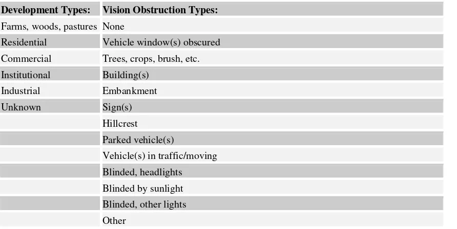
weather (snow, rain, sleet, fog, cloudy, clear), and others that may obstruct vision
(sunlight, trees, buildings, and vehicles).
Dependent variables
Consistent with the objectives of this study, the dependent variables are the severity of
accidents and the cost of accidents. For severity, we distinguish between four types of
crashes. They are those that cause fatalities, incapacitating injuries, evident but not
incapacitating injuries, and possible injuries. A separate model is developed to explain each
of the four types of severe accidents. For the cost of accidents, we use two dependent
variables. The first is the estimate of property damage cost in the police accident reports.
This property damage cost is approximate. However, under the assumption that errors in this
cost are independent of the explanatory variables, we can use it in our equations. Police
officers are required to file a complete accident report providing damage estimates if the
property damage is at least $1,000 or if an injury occurred. Our data show many property
11
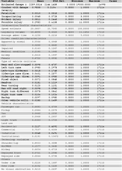
Table 2: Descriptive Statistics
Variable Mean Std.Dev. Minimum Maximum Cases
Estimated damage $ 2259.3314 2144.1438 0.0000 19000.0000 16993 Crashes with damage 0.9535 0.2106 0.0000 1.0000 17116 Severity
Fatalities 0.0010 0.0315 0.0000 1.0000 17116 Incapacitating 0.0045 0.0728 0.0000 3.0000 17116 Evident injury 0.0511 0.2465 0.0000 4.0000 17116 Possible injury 0.2952 0.6138 0.0000 11.0000 17116 Intersection/Traffic characteristics
Speed estimate 20.0807 15.7065 0.0000 100.0000 16986 Log(daily volume) 10.4050 0.4323 8.8209 11.1452 17110 Average amber time 4.1236 0.2216 3.0000 5.0500 17110 Driver condition/characteristics
Apparently normal 0.5566 0.4968 0.0000 1.0000 17110 Ill 0.3200 0.4665 0.0000 1.0000 17110 Impaired 0.0163 0.1267 0.0000 1.0000 17110 Medical condition 0.2180 0.1460 0.0000 1.0000 17110 Asleep 0.0416 0.1997 0.0000 1.0000 17110 Female 0.4722 0.4992 0.0000 1.0000 17110 Type of vehicle collision
Rear end slow/stopped 0.3398 0.4737 0.0000 1.0000 17116 Left turn same 0.0983 0.2978 0.0000 1.0000 17116 Left-turn different 0.0315 0.1748 0.0000 1.0000 17116 Sideswipe same direc. 0.0601 0.2377 0.0000 1.0000 17116 Sideswipe opp. direc. 0.0091 0.0950 0.0000 1.0000 17116 Fixed object 0.0072 0.0845 0.0000 1.0000 17116 Head-on 0.0151 0.1219 0.0000 1.0000 17116 Rear turning 0.0123 0.1101 0.0000 1.0000 17116 Ran off road right 0.0098 0.0983 0.0000 1.0000 17116 Right turn different 0.0075 0.0862 0.0000 1.0000 17116 Right turn same 0.0106 0.1026 0.0000 1.0000 17116 Backup 0.0097 0.0980 0.0000 1.0000 17116 Other vehicle colli. 0.0283 0.1659 0.0000 1.0000 17116 Vehicle characteristics
Passenger car 0.6683 0.4709 0.0000 1.0000 17110 Pickup 0.0984 0.2979 0.0000 1.0000 17110 Van 0.0440 0.2050 0.0000 1.0000 17110 SUV 0.0968 0.2957 0.0000 1.0000 17110 Light truck 0.0303 0.1715 0.0000 1.0000 17110 Land use
Residential 0.2127 0.4092 0.0000 1.0000 17116 Commercial 0.7537 0.4309 0.0000 1.0000 17110 Industrial 0.0048 0.0691 0.0000 1.0000 17116 Institutional 0.0191 0.13672 0.0000 1.0000 17110 Technology variables
Shoulder/lap 0.8933 0.3088 0.0000 1.0000 17116 RLCPRES 0.1577 0.3645 0.0000 1.0000 17110 Airbag 0.6654 0.4719 0.0000 1.0000 17110 Deployed front 0.0721 0.2586 0.0000 1.0000 17110 Deployed side 0.0064 0.0799 0.0000 1.0000 17110 Others
Descriptive statistics
The descriptive statistics in Table 2 provide some information about the data. These
statistics show that those involved in the crashes were mostly men (52.78%) and appeared
normal (55.66%). However, a sizable percentage (21.80%) had medical conditions and
32.00% were ill. Those impaired by drugs and/or alcohol accounted for only 1.63% of the
crashes and a driver falling asleep behind the wheel accounted for 4.16% of the crashes.
An observation from the table is that 75.37% of the crashes occurred where the
predominant land use is commercial and 21.27% occurred where the predominant land use
is residential. Very few crashes occurred near where the major land use is industrial or
institutional. This distribution of where the crashes occurred could reflect prior
determination by traffic engineers concerning where to locate traffic lights. Since
commercial land uses generate a lot of vehicular traffic, it is common to locate traffic lights
near them. The same can be said of residential land use, though to a lesser extent.
A further observation is that 95.35% of the crashes involved property damage
costing $2,259.33 on the average, and 29.52% of the crashes involved possible injuries. The
data also show that very few accidents were fatal (0.10%), incapacitating (0.45%), or
involved evident injury (5.11%). In short, most of these crashes were minor. One reason for
this may be the low average estimated traveling speed of 20.08 miles per hour for the
vehicles in the crashes and 66.54% of these vehicles having airbags. Also, it may be because
89.33% of the vehicle occupants wore seatbelts. Furthermore, in 7.21% of the vehicles, the
airbags in the front passenger compartment deployed possibly reducing injuries to the driver
and front-seat occupants, while in 0.64% the side airbags deployed. This latter percentage
could indicate the most severe crashes. In fact, since this percentage is very close to that for
fatalities it is possible that both percentages show the same type of crash.
Due to the preponderance of passenger cars in traffic streams, we would expect that
most of the crashes would involve passenger cars. Indeed, this is the case as the data reveals.
The data shows that though various types of vehicles were involved in crashes, most
(66.83%) were passenger cars, 9.84% were pickups, 9.68% were sports utility vehicles,
4.4% were vans, and 3.3% were light trucks. The rest, 5.8% included single unit trucks,
tractor-trailers, taxicabs, motorcycles, and school buses, etc.
Because the focus of the study is on vehicular crashes, the data does not show
13
show that 33.98% of the intersection crashes involved running into the back of a slowed or
stopped vehicle, 9.83% involved vehicles making a left in the same roadway, 6.01%
involved sideswiping a vehicle in the same direction, while 3.15% involved vehicles turning
left on different roadways. Each of the other entries in the table shows a percentage that is
less than three percent.
Correlations
The data was analyzed using various statistical methods including correlation to establish
relationships among the independent variables. This is particularly important to identify
linear dependencies among the variables that could seriously affect the reliability of the
estimated coefficients. Appendix A shows the correlations between the independent
variables. Clearly, most of these correlations are very low suggesting that linear
dependencies would not be a problem in using these variables in the equations to be
estimated. However, close observation reveals a sizable positive correlation between red
light cameras and traffic volume. Since higher traffic volumes are generally associated with
minor accidents because speed tends to be low, we should expect some relationship between
red light cameras and minor accidents. In the next section, we will examine if this
relationship indeed exists when other confounding variables are accounted for. Interestingly,
there is a negative correlation between female drivers and the reporting of an accident being
related to falling asleep or a medical condition.
4. ANALYSIS OF CRASH-LEVEL SEVERITY
This section analyzes factors that can predict the most severe injury sustained by all
involved in a crash. Milton and Mannering (1998) argue that since most accident frequency
data are over-dispersed, the appropriate model to use is the negative binomial model.
However, in this section we categorize individual accidents by severity and perform analysis
to determine the factors that explain the severity category. For example, the occurrence of a
fatal accident or an accident involving property damage is recorded as one and
non-occurrence as a zero. Because these non-occurrences are the dependent variables in our
equations, negative binomial models are inappropriate. Because the dependent variable is
dichotomous, we use probit and logit equations to estimate an equation for each type of
In addition, there are very few fatal crashes in the data; therefore, they are combined
with those that result in incapacitating injuries and one equation estimated for them. In all,
two equations are estimated for crash severity and they are: 1) a probit model for fatal and
incapacitating crashes, and 2) a probit model for evident injury. These equations are of the
form,
) 1 (
β
X Y=
Where Y is the dependent variable, X is a subset of the independent variables in Table 2 and
β is a vector of the coefficients to be estimated. These independent variables are the
characteristics of signalized intersections, traffic and road characteristics, land use
characteristics, driver characteristics, technology, and environmental variables.
Results
Fatal and incapacitating injuries
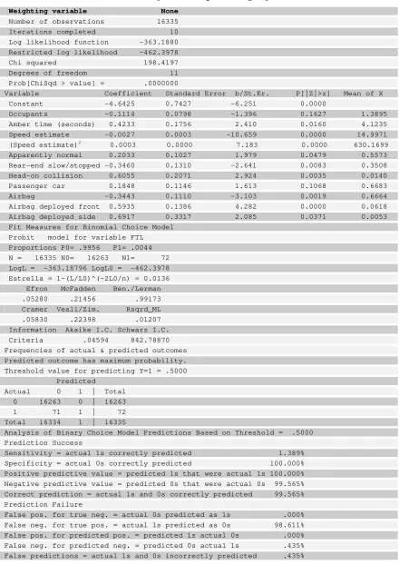
Table 3 shows the maximum likelihood estimates of the coefficients of the equation for the
combined fatal and incapacitating injuries from vehicle crashes. The fit statistics show that
the model fits the data relatively well. At the 0.5 threshold level (i.e., predict that fatalities
and incapacitating injuries equal to one if the fitted probability of these injuries occurring is
greater than 0.5), 99.67% of the actual ones and zeroes in the dependent variable are
correctly predicted. However, it is worth noting that with this threshold, the model correctly
predicts the zeroes better than it predicts the ones. For example, while it correctly predicts
99.565% of the zeroes, it incorrectly predicts 98.61% of the ones. These results show that
the data is quite unbalanced with many zeroes. In fact, our data has 72 crashes involving
fatal or incapacitating injuries (i.e., probability = 0.0055) coded as ones compared to 16,263
crashes coded as zeroes that did not result in these injuries. These levels of prediction
notwithstanding, the results provide useful information to explain crashes that result in fatal
and incapacitating injuries.
The effect of technology variables on fatal and incapacitating injuries: From the
coefficients in Table 3, some information can be gleaned about the effect of technology
variables on crashes that result in fatalities and incapacitating injuries. These technology
variables are the presence of airbags in the vehicles involved in the crashes, front airbag
15
confirms the commonly accepted notion that airbags reduce fatalities and incapacitating
injuries. On the other hand, when we examine the coefficients of airbag deployment, the
opposite results are obtained. Here, the coefficients of both the front and side airbags
deploying are positive and statistically significant at the 0.0000 and 0.0371 levels
respectively. These positive coefficients suggest that when the front and side airbags deploy
in crashes, they could result in incapacitating injuries and possibly fatalities.
The relative contributions of the technology variables to incapacitating injuries and
fatalities from intersection crashes are obtained by examining their marginal effects. These
marginal effects are presented below. Clearly, they show that the marginal effect of the side
airbag deploying versus not deploying is not statistically significant. On the other hand, the
marginal effects of the front airbag deploying and there being an airbag in a vehicle involved
in a crash at an intersection are statistically significant. The sizes of these marginal effects
show that when a front airbag deploys it may increase the probability of injuries and
fatalities occurring more than the reduction in this probability when there is an airbag in a
Table 3: Binomial Probit: Fatality and Incapacitating Injuries
Weighting variable None
Number of observations 16335 Iterations completed 10 Log likelihood function -363.1880 Restricted log likelihood -462.3978 Chi squared 198.4197 Degrees of freedom 11 Prob[ChiSqd > value] = .0000000
Variable Coefficient Standard Error b/St.Er. P[|Z|>z] Mean of X Constant -4.6425 0.7427 -6.251 0.0000
Occupants -0.1114 0.0798 -1.396 0.1627 1.3895 Amber time (seconds) 0.4233 0.1756 2.410 0.0160 4.1235 Speed estimate -0.0027 0.0003 -10.659 0.0000 14.9971 (Speed estimate)2 0.0003 0.0000 7.183 0.0000 630.1699
Apparently normal 0.2033 0.1027 1.979 0.0479 0.5573 Rear-end slow/stopped -0.3460 0.1310 -2.641 0.0083 0.3508 Head-on collision 0.6055 0.2071 2.924 0.0035 0.0140 Passenger car 0.1848 0.1146 1.613 0.1068 0.6683 Airbag -0.3443 0.1110 -3.103 0.0019 0.6664 Airbag deployed front 0.5935 0.1386 4.282 0.0000 0.0618 Airbag deployed side 0.6917 0.3317 2.085 0.0371 0.0053 Fit Measures for Binomial Choice Model
Probit model for variable FTL Proportions P0= .9956 P1= .0044 N = 16335 N0= 16263 N1= 72 LogL = -363.18796 LogL0 = -462.3978 Estrella = 1-(L/L0)^(-2L0/n) = 0.0136 Efron McFadden Ben./Lerman .05280 .21456 .99173 Cramer Veall/Zim. Rsqrd_ML .05830 .22398 .01207 Information Akaike I.C. Schwarz I.C. Criteria .04594 842.78870 Frequencies of actual & predicted outcomes Predicted outcome has maximum probability. Threshold value for predicting Y=1 = .5000 Predicted
Actual 0 1 | Total 0 16263 0 | 16263 1 71 1 | 72 Total 16334 1 | 16335
Analysis of Binary Choice Model Predictions Based on Threshold = .5000 Prediction Success
Sensitivity = actual 1s correctly predicted 1.389% Specificity = actual 0s correctly predicted 100.000% Positive predictive value = predicted 1s that were actual 1s 100.000% Negative predictive value = predicted 0s that were actual 0s 99.565% Correct prediction = actual 1s and 0s correctly predicted 99.565% Prediction Failure
17
Mean Standard. Error t-value Probability
Airbag present in vehicle
-0.0022 0.0008 -2.631 0.0085
Front airbag deployed
0.0071 0.0030 2.409 0.0160
Side airbag deployed 0.0105 0.0104 1.015 0.3103
Types of accidents vs. fatal and incapacitating injuries: Types of accidents also have
significant effects on fatalities and incapacitating injuries. Two types of crashes are
examined here. They are running into the back of a slowed or stopped vehicle, and head-on
collision. Both types of crashes have opposite and statistically significant effects on fatal and
incapacitating injuries. Running into the back of a slowed or stopped vehicle at an
intersection is negatively associated with suffering incapacitating injuries and fatalities,
showing that these crashes are generally not serious. On the other hand, a head-on collision
is a very serious crash and it is positively associated with fatalities and incapacitating
injuries. Examining the marginal effects of these types of crashes, we observe that when an
intersection crash involves running into the back of a slowed or stopped vehicle, its marginal
effect on the probability of fatality and incapacitating injuries occurring is negative
(-0.0016) and statistically significant (0.0034). Contrariwise, when the crash involves a
head-on collisihead-on, its marginal effect (0.0080) is not statistically significant (0.1304).
Driver condition vs. fatal and incapacitating injuries: Driver condition at the time of a
crash also affects fatality and incapacitating injuries. We noted this in the data section; here
we consider it explicitly in modeling fatal and incapacitating injuries. While the data
provides a variety of information about driver condition, only one is considered in Table 3
and this is if the driver involved in the crash appeared normal. The log-likelihood estimation
did not converge to a solution when other descriptors of driver condition were included in
the model. The results of the estimation in Table 3 show that those involved in crashes that
involved fatalities and incapacitating injuries appeared normal. The estimated coefficient of
this driver condition and its associated probability are respectively 0.2033 and 0.0479. And,
its marginal effect of 0.0011 with a level of significance of 0.0464 shows that apparently
that leads to fatalities and incapacitating injuries. This suggests that such crashes may be due
to drivers who do not appear normal or who may have some medical problems.
Intersection and traffic characteristics vs. fatal and incapacitating injuries: Four variables
are used to capture the effects of intersection and traffic characteristics on crashes that result
in fatalities and injuries. They are the type of vehicle involved in the crash (represented by
passenger car), the estimated speed of the vehicle in the crash, the square of this estimated
speed, and amber time setting. The results show that the coefficient of passenger car, though
positive, is not statistically significant. Its probability of 0.1068 is outside the commonly
acceptable range, i.e., p < 0.10. Thus, we cannot say that when passenger cars are involved
in crashes at signalized intersections they would be associated with more fatalities and
incapacitating injuries than other vehicles. When also we examine the amber time settings at
signalized intersection, it can be said that they appear to be associated with high levels of
crashes that result in fatalities and incapacitating injuries. Here, we observe that the
coefficient of amber time is 0.4233 with a probability of 0.0160, which is statistically
significant. However, the marginal effect of amber time is 0.0022 (probability = 0.0185) and
shows that increasing it by one second would increase by 0.22% the probability of a crash
occurring that involves fatalities and incapacitating injuries.
The effect of estimated travel speed on crashes involving fatalities and incapacitating
injuries is examined with two variables, one linear and the other quadratic. The results show
that both variables have coefficients that are opposite in signs and that are highly significant
(probability < 0.0000). While the linear speed term has a negative coefficient, the quadratic
term has a positive coefficient. These coefficients imply that as estimated travel speed
increases there would be an initial reduction in crashes resulting in fatalities and
incapacitating injuries. This could occur if it increases traffic flow and reduces stop-and-go
operations. However, at some point an increase in speed would increase the probability of
crashes resulting in fatalities and incapacitating injuries.
Evident injury
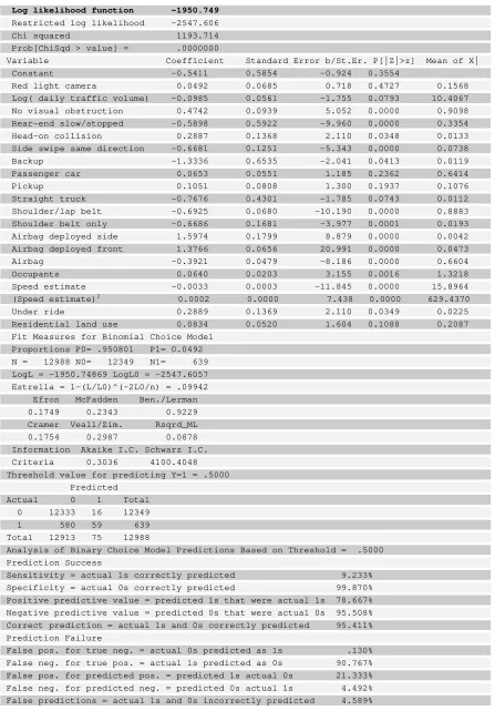
Table 4 shows the maximum likelihood estimate of crashes that involved evident injury.
Here, we removed from the data all crashes that involved fatal, incapacitating, and possible
19
0.0000. We also observe that at the 5% threshold level the model predicts 99.87% of the
actual zeroes and 9.233% of the actual ones, which reflects the unbalanced nature of the
data. Specifically, the data contains 4.92% of crashes that resulted in evident injuries.
Combined, at this threshold level, the model correctly predicts 95.411% of the actual ones
and zeroes.
The effect of technology variables on evident injury: The technology variables considered in
this equation include the presence of red light cameras at intersections, drivers’ use of
shoulder and lap belts, and use of only lap belt at the time of the crash. Others are the
presence of an airbag in a vehicle involved in a crash, front airbag deployed, and side
airbags deployed. Obviousl,y from the table the presence of a red light camera at an
intersection is not related to crashes that result in evident injuries. This is quite surprising
since red light cameras are touted for reducing crashes at intersections, particularly severe
crashes that cause injuries. However, it is consistent with what Burkey and Obeng (2004)
found in their study of red light cameras using a subset of data included in this study.
The relationship between the presence of airbags in vehicles and evident injury is
negative and statistically significant and similar to what we found between crashes that
result in fatal and incapacitating injuries and airbags. The coefficient of the presence of an
airbag in a vehicle is -0.3932 and it is significant at the 0.0000 level. Therefore, the
probability of crashes occurring at signalized intersections that result in evident injuries
could reduce if the vehicles had airbags. However, when the airbags deploy they do not have
the same negative effect on evident injuries as the presence of an airbag in a vehicle.
Whether the airbag deploys in front or on the side, its effect is to increase the probability of
an evident injury occurring. This is quite clear from the coefficients of 1.5974 (probability =
0.0000) and 1.3766 (probability = 0.0000) for side and front airbags deploying respectively.
The marginal effects of the presence of an airbag in a vehicle, and front and side airbags
deploying also are statistically significant and are shown below. These marginal effects
show that when either the front or the side airbag deploys the probability of evident injury
occurring is far larger than the decrease in the probability of an evident injury occurring in a
Table 4 – Binomial Probit Model of Evident Injury
Log likelihood function -1950.749
Restricted log likelihood -2547.606 Chi squared 1193.714 Prob[ChiSqd > value] = .0000000
Variable Coefficient Standard Error b/St.Er. P[|Z|>z] Mean of X| Constant -0.5411 0.5854 -0.924 0.3554
Red light camera 0.0492 0.0685 0.718 0.4727 0.1568 Log( daily traffic volume) -0.0985 0.0561 -1.755 0.0793 10.4067 No visual obstruction 0.4742 0.0939 5.052 0.0000 0.9098 Rear-end slow/stopped -0.5898 0.5922 -9.960 0.0000 0.3354 Head-on collision 0.2887 0.1368 2.110 0.0348 0.0133 Side swipe same direction -0.6681 0.1251 -5.343 0.0000 0.0738 Backup -1.3336 0.6535 -2.041 0.0413 0.0119 Passenger car 0.0653 0.0551 1.185 0.2362 0.6414 Pickup 0.1051 0.0808 1.300 0.1937 0.1076 Straight truck -0.7676 0.4301 -1.785 0.0743 0.0112 Shoulder/lap belt -0.6925 0.0680 -10.190 0.0000 0.8883 Shoulder belt only -0.6686 0.1681 -3.977 0.0001 0.0193 Airbag deployed side 1.5974 0.1799 8.879 0.0000 0.0042 Airbag deployed front 1.3766 0.0656 20.991 0.0000 0.0473 Airbag -0.3921 0.0479 -8.186 0.0000 0.6604 Occupants 0.0640 0.0203 3.155 0.0016 1.3218 Speed estimate -0.0033 0.0003 -11.845 0.0000 15.8964 (Speed estimate)2 0.0002 0.0000 7.438 0.0000 629.4370
Under ride 0.2889 0.1369 2.110 0.0349 0.0225 Residential land use 0.0834 0.0520 1.604 0.1088 0.2087 Fit Measures for Binomial Choice Model
Proportions P0= .950801 P1= 0.0492 N = 12988 N0= 12349 N1= 639 LogL = -1950.74869 LogL0 = -2547.6057 Estrella = 1-(L/L0)^(-2L0/n) = .09942 Efron McFadden Ben./Lerman 0.1749 0.2343 0.9229 Cramer Veall/Zim. Rsqrd_ML 0.1754 0.2987 0.0878 Information Akaike I.C. Schwarz I.C. Criteria 0.3036 4100.4048 Threshold value for predicting Y=1 = .5000 Predicted
Actual 0 1 Total 0 12333 16 12349 1 580 59 639 Total 12913 75 12988
Analysis of Binary Choice Model Predictions Based on Threshold = .5000 Prediction Success
Sensitivity = actual 1s correctly predicted 9.233% Specificity = actual 0s correctly predicted 99.870% Positive predictive value = predicted 1s that were actual 1s 78.667% Negative predictive value = predicted 0s that were actual 0s 95.508% Correct prediction = actual 1s and 0s correctly predicted 95.411% Prediction Failure
21
MARGINAL
EFFECT STD. ERR T-VALUE PROB.
Shoulder and lap -0.0695 0.0102 -6.844 0.0000 Shoulder belt only -0.0217 0.0027 -8.147 0.0000 Airbag deployed front 0.2392 0.0198 12.096 0.0000 Airbag deployed side 0.3339 0.0667 5.010 0.0000
Airbag -0.0027 0.0037 -7.251 0.0000
Two other technology variables whose relationships with evident injury we
examined are shoulder and lap belts. When used together, these belts have negative
relationships with there being evident injuries in crashes at intersections. The coefficient of
using lap and shoulder belts together is -0.6925 with a probability of 0.0000. Similarly,
when shoulder belts are used alone they reduce the probability of evident injuries occurring
in crashes at signalized intersections. The coefficient of using shoulder belts alone is -0.6686
with a probability of 0.0001. Although these coefficients are very close, their marginal
effects in the above table show that the injury reduction effect of using shoulder and lap
belts together is more than three times the effect of using a shoulder belt alone. To be exact,
when shoulder and lap belts are used the probability of sustaining evident injury in a crash
reduces by 6.95% (probability = 0.0000), compared to a reduction of 2.17% (probability =
0.0000) in sustaining evident injury in an accident at an intersection.
Combining these results we consider a typical automobile user, a driver wearing a
combined shoulder and lap belt and driving a vehicle equipped with front and side airbags
that deploy during a crash at a signalized intersection. The marginal effects of the
technology variables show that such a typical automobile driver would have a 50.09%
chance of sustaining an evident injury. If the same driver used only the shoulder belt, the
probability of him/her sustaining evident injury becomes 54.87%. If the vehicle did not have
a side airbag the probability of an evident injury occurring would reduce to 16.70%.
Types of accidents vs. evident injuries: Evident injuries may also be due to the types of
crashes that occur. Though our data contain many types of crashes, we focus only on those
for which we obtained statistically significant coefficients. Three types of accidents
qualified to be included in the model of evident injury and two had negative and statistically
significant coefficients. These two are crashing into the back of a slowed or stopped vehicle
and backing up, and their respective coefficients are -0.6681 (0.0000) and –1.3336 (0.0413),
intersection resulting in evident injury is smaller when it involves running into the back of a
slowed or stopped vehicle, or when the crash results from a vehicle backing up. These
results are also borne out when we examine the marginal effects of these types of crashes.
Such an examination leads to the table below, which shows that the reduction in the
probability of evident injury is larger than occurs from side swiping a vehicle that is moving
in the same direction.
MARGINAL
EFFECT STD. ERR T-VALUE PROB.
Back of slowed/stopped vehicle -0.0302 0.0027 -11.356 0.0000
Head on collision 0.0225 0.0136 1.660 0.0969
Side swipe vehicle in same direction -0.0235 0.0024 -9.651 0.0000
While both types of crashes are negatively related to evident injury, Table 4 and
above table show that head on collisions are positively associated with sustaining an injury.
The coefficient of head on collision is 0.2887 and it is significant at the probability level of
0.0348. However, the probability of the marginal effect of head on collision is very weak,
leading us to surmise that there is not strong evidence to suggest that head on crashes at
signalized intersections are not strongly related to evident injury. This may be because these
types of crashes seldom occur particularly in an environment where raised medians are used
at signalized intersections to separate traffic flowing in opposite directions.
Type of vehicle versus evident injury: To examine the impact of the type of vehicle involved
in a crash on evident injury we included three types of vehicles in the model. They are
passenger cars, pickups, and straight trucks. Both passenger cars and pickups have positive
coefficients in the model, but these coefficients are not statistically significant. This shows
that we cannot be confident that evident injury would be observed when these two types of
vehicles are involved in crashes. Contrary to these results we find that the coefficient of a
straight truck is -0.7676 and its level of significance of 0.0743 is very weak, just as is its
marginal effect. Specifically, the marginal effect of a straight truck is 0.0068 with a level of
significance of 0.2288. Together these results show that type of vehicle does not have a
statistically significant effect on crashes at a signalized intersection that result in evident
23
Traffic volume and speed vs. evident injury: Table 4 also shows the effects of traffic volume
and speed on the probability of evident injuries occurring in crashes at signalized
intersections. The coefficient of traffic volume is –0.0985 with a significance level of
0.0793, which shows that its relationship with evident injuries is very weak. However, when
we examine the effect of estimated speed the vehicle was traveling when the accident
occurred, its linear and quadratic terms are highly statistically significant. The coefficient of
the linear and quadratic terms are –0.0033 (0.0000) and 0.0002 (0.0000) respectively, where
the terms in parentheses are the probabilities. As we have argued in previous discussions,
the negative coefficient of the linear term shows that the probability of evident injury
occurring is low when estimated speed is high, while the coefficient of the quadratic term
shows that beyond some point an increase in estimated speed would be associated with an
increase in the probability of evident injury occurring.
Type of land use and evident injury: The effect of land use on evident injury is also in Table
4. Here, the considered land use is residential and it is found that it does not have a
statistically significant effect on evident injury. Though its coefficient is positive, its level of
significance of 0.1088 shows this coefficient is not different from a zero. Thus, crashes
involving evident injury are found everywhere and not confined to specific places or where
some predominant land uses occur.
Other factors vs. evident injury: Besides the above results, crashes that involve under rides
result in evident injury. The coefficient of this variable is 0.2889 and its level of significance
is 0.0349. Similarly, when a crash is a result of no visual obstruction it results in evident
injuries. The coefficient of no visual obstruction is 0.4742 with a probability of 0.0000. It
follows that crashes at intersections that result in evident injuries cannot be attributed to
visual obstructions.
5. DETERMINANTS OF INJURIES IN TWO-VEHICLE CRASHES
The discussions in the previous section were concerned with fatalities and incapacitating
injuries, and evident injuries. In those discussions, we considered all types of crashes and
did not distinguish between single car and multiple car crashes. In this section, we consider
the most common type of crashes at signalized intersections, crashes involving two vehicles.
of severity using the KABCO method. The fatalities and severe injuries (Type A) occurred
so rarely in the data set that they were combined with evident injuries and non-disabling
injuries (Type B) into a category called ‘Severe.” Possible injuries (Type C) were examined
for comparison. This process yielded 6,188 events with 12,376 vehicles involved containing
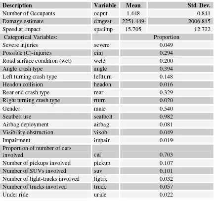
17,922 occupants. The proportions of persons who had severe and possible injuries are 4.9%
and 29.4% respectively. Of the types of accidents recorded, 39.4% involved angle crashes,
14.8% left-turning vehicles, 1.6% head-on collisions, 32.9% rear-ending a slow or stopped
vehicle and 2.0% right-turning vehicles. About 54% of the crashes involved male drivers,
98% of the drivers wore seatbelts during the crash, and 1.9% of the drivers were impaired.
For 8.1% of the crashes, air bags deployed, and 5% involved visibility obstruction. Table 5
presents descriptive statistics for the explanatory variables in the study of two vehicle
crashes. Using this data we analyzed the factors that influence the number of severe (K, A,
B) and possible (C) injuries that occur in two-vehicle crashes. These factors include the
characteristics of the vehicle containing the occupants who suffered injuries as well as the
characteristics of the other vehicle involved in the crash. Of key interest here are the
estimated speeds of both vehicles at impact and the types of vehicles involved.
To focus on the most common occurrences with a relatively simple model, we
restricted attention to accidents involving cars, pickups, SUVs, minivans, and “single unit
trucks.” These single unit trucks include many types of delivery trucks that have two axles.
Examining all of the possible combinations of these vehicle types would require 20 different
pairings to be examined. To reduce this to 12 categories, pickups and minivans were
combined into one category because of their similar weights.
The model
Again, recall that the number of injuries of each type is a count variable. So, we employ
Poisson regression models to analyze two-vehicle crashes. However, it would be improper
to ignore the fact that the number of severe injuries and the number of minor injuries
occurring in the same vehicle are related. A method that considers this relationship is
therefore needed. Some authors have used Seemingly Unrelated Regression (SUR) type
model tailored for count data in analyzing this relationship (King, 1989; Winkelmann,
2000). A relatively new approach is the bivariate Poisson constructed using a
25
Table 5: Descriptive Statistics of Data for Two-Vehicle Crashes
Description Variable Mean Std. Dev.
Number of Occupants ocpnt 1.448 0.841
Damage estimate dmgest 2251.449 2006.815
Speed at impact spatimp 15.705 12.722
Categorical Variables: Proportion
Severe injuries severe 0.049
Possible (C)-injuries cinj 0.294
Road surface condition (wet) wet3 0.200
Angle crash type angle 0.394
Left turning crash type leftturn 0.148
Headon collision headon 0.016
Rear end crash type rear 0.329
Right turning crash type rturn 0.020
Gender male 0.540
Seatbelt use seatbelt 0.982
Airbag deployment airbag 0.081
Visibility obstruction visob 0.049
Impairment impair 0.019
Proportion of number of cars
involved car 0.703
Number of pickups involved pickup 0.107
Number of SUVs involved suv 0.101
Number of light-trucks involved ligtrk 0.032
Number of trucks involved truck 0.057
Under ride uride 0.022
To understand this technique let X1, X2, and X3 be independent Poisson random
variables. We can construct conceptual models in the standard (log-link) way, modeling the
expected values of the Xi as X Bi i, {1, 2,3}
i e i
λ = ∈ . Then, both {X= X1 + X3, Y= X1 + X3}
follow a bivariate Poisson distribution. The joint probability density function of this
distribution is
min( , ) 3
1 2
1 2 3 0
1 2
( , ) exp( ( )) !
! ! k x y x y k x y
P X x Y y k
k k x y
λ λ λ
λ λ λ
λ λ = ⎛ ⎞ ⎛ ⎞⎛ ⎞ = = = − + + ⎜ ⎟⎜ ⎟ ⎜ ⎟ ⎝ ⎠⎝ ⎠ ⎝ ⎠
∑
This formulation is convenient because it explicitly allows for a relationship between X and
Y, namely, cov (X, Y) = λ3. If this covariance is zero, the estimation reduces to the product
(1997)). It has been shown that a misspecification of a binomial Poisson as a double Poisson
model will cause the model’s parameters to be overestimated (Karlis & Ntzoufras, 2003).
Application of this equation requires estimating three equations jointly, i.e., two
“independent” equations for severe (fatal and incapacitating injuries) and evident injuries,
and a covariance equation showing the interrelatedness of these two equations.3 The two
“independent” equations explaining severe and possible injuries in the first vehicle in a
two-vehicle crash use three types of explanatory variables. First, is a set of indicator variables to
account for the types of vehicles in two-vehicle accident. There were twelve possible
accident types (e.g., the first vehicle is a car and the second vehicle is SUV), and we created
interaction variables for them and used a car-car accident as the reference category,
therefore omitting it from the estimation. These interaction variables measure the relative
impact of a collision in comparison to riding in a car and being in an accident where the
other vehicle is also a car. For reference, there were 3,090 car-car accidents (7,180 vehicles)
involving 304 severe injuries and 1,941 C injuries for the 8,914 occupants of the vehicles.
This implies mean risk rates of 0.0341 and 0.2177 per occupant. The coefficients of the
interaction variables should be understood in relation to these values. The third equation,
which constructs the covariance between the two types of injury severity, contains the
estimated speed of both vehicles at impact and the natural logarithm of the number of
occupants is used as the exposure variable.
Diagnostics and Goodness of Fit
The most common problem facing Poisson models is over-dispersion. Since the Poisson is a
single parameter distribution, such that the mean is equal to the variance, one must check for
a violation of this assumption. Over-dispersion is particularly problematic because if the
variance is much larger than the mean type one errors can result because of underestimated
standard errors. In the two-vehicle crashes, the means and variances are very close for each
of the two dependent variables. From our data, the mean of the severe injuries is 0.049, and
the variance of the residuals is 0.056. For the possible injuries variable the mean is 0.294,
and the variance of the residuals is 0.355. These small amounts of over-dispersion will not
affect the results in this paper because the bivariate Poisson’s standard errors are estimated
via a bootstrap method. The standard errors reported here were generated with 200