Markets Evolution After the Credit Crunch

Markets Evolution After the Credit

Crunch

Bianchetti, Marco and Carlicchi, Mattia

19 December 2012

Markets Evolution After the Credit Crunch

Marco Bianchetti

Market Risk Management, Intesa Sanpaolo, Piazza Paolo Ferrari, 10, 20121 Milan, Italy,

marco.bianchetti[AT]intesasanpaolo.com

Mattia Carlicchi

Market Risk Management, Intesa Sanpaolo, Piazza Paolo Ferrari, 10, 20121 Milan, Italy,

mattia.carlicchi[AT]intesasanpaolo.com

19 December 2012

Abstract

We review the main changes in the interbank market after the financial crisis started in August 2007. In particular, we focus on the fixed income market and we analyse the most relevant empirical evidences regarding the divergence of the existing basis between interbank rates with different tenor, such as Libor and OIS. We also discuss a qualitative explanation of these effects based on the consideration of credit and liquidity variables. Then, we focus our attention on the diffusion of collateral agreements among OTC derivatives market counterparties, and on the consequent change of paradigm for pricing derivatives. We illustrate the main qualitative features of the new market practice, called CSA discounting, and we point out the most relevant issues for market players associated to its adoption.

Keywords: crisis, liquidity, credit, counterparty, risk, fixed income, Libor, Euribor, Eonia, OIS – Libor basis, yield curve, forward curve, discount curve, single curve, multiple curve, collateral, CSA discounting, no arbitrage, pricing, interest rate derivatives, FRA, swap, OIS, basis swap, forward rate, CDS spread, ECB monetary policy, ISDA.

JEL Classifications: E43, G12, G13.

Acknowledgements and disclaimer

A version of this paper appears as a chapter in “Interest Rate Modelling After the Financial Crisis”, editors M. Bianchetti and M. Morini, Risk Books, 2013.

The authors gratefully acknowledge fruitful interactions with M. Morini and many colleagues at Intesa Sanpaolo and Banca IMI.

Table of Contents

1. Introduction ... 3

2. The Interbank Market After the Financial Crisis ... 3

2.1. Euribor – Eonia Basis ... 4

2.2. FRA Rates versus Forward Rates ... 7

2.3. Basis Swaps ... 11

2.4. The Credit and Liquidity Risk Components ... 15

2.5. A Simple Credit Model ... 19

3. Collateralization and CSA Discounting ... 21

3.1. Collateral Diffusion ... 21

3.2. Collateral Mechanics... 23

3.3. CSA Discounting ... 24

3.4. Market Quotes ... 26

3.5. Market Practice and P&L Impacts ... 28

3.6. Issues of CSA Discounting... 29

3.6.1. Collateral and Liquidity Issues ... 29

3.6.2. Accounting Issues ... 29

3.6.3. IT Issues ... 30

3.6.4. Risk Management Issues ... 30

3.6.5. Management Issues ... 32

3.6.6. The Role of Quants ... 32

4. Conclusions ... 32

1. Introduction

The financial crisis begun in the second half of 2007 has triggered, among many consequences, a deep evolution phase of the classical framework adopted for trading derivatives. In particular, credit and liquidity risks were found to have macroscopical impacts on the prices of financial instruments, both plain vanillas and exotics. The market has learnt the lesson and persistently shows such effects. These are clearly visible in the market quotes of plain vanilla interest rate instruments, such as Deposits, Forward Rate Agreements (FRA), Swaps (IRS) and options (European Caps, Floors and Swaptions). Since August 2007, the primary interest rates of the interbank market, e.g. Libor, Euribor, Eonia, and Federal Funds rate1, display large basis spreads that have raised up to 200 basis points. Similar divergences are also found between FRA rates and the forward rates implied by two consecutive Deposits, and similarly, among Swap rates with different floating leg tenors (Basis Swaps).

After the financial crisis, the standard no-arbitrage framework adopted to price derivatives, developed over forty years following the Copernican Revolution of Black and Scholes (1973) and Merton (1973), became obsolete. Familiar relations described on standard textbooks (see e.g. Brigo and Mercurio 2006, Andersen and Piterbarg 2012, Hull 2008), such as the basic definition of forward interest rates, or the swap pricing formula, had to be abandoned. Also the fundamental idea of the construction of a single risk free yield curve, reflecting at the same time the present cost of funding of future cash flows and the level of forward rates, has been ruled out. The financial community has thus been forced to start the development of a new theoretical framework, including a larger set of relevant risk factors, and to review from scratch the no-arbitrage models

used on the market for derivatives’ pricing and risk analysis. A relevant feature of the post-crisis market is given by the consideration of collateral agreements in the pricing framework of OTC trades.

The paper is organized as follows. In section 2 we report the main changes and market evidences that characterize the most relevant interest rates of the interbank market since the explosion of the financial crisis. In particular, we focus on the EUR market and we analyze the relation between Euribor and Eonia market rates with different tenors, as observed in market quotations of Deposits, FRA, Swaps, Basis Swaps and Overnight Indexed Swaps (OIS). We argue that the financial crisis has sparked market liquidity and credit risk perception, that has been promptly reflected in the interest rates dynamics through increased and differentiated risk premia. We present a qualitative analysis of the Euribor – Eonia basis where we highlight the impacts of the credit and liquidity risk factor by introducing synthetic proxies that gauge the evolution of these two components during the period Jan. 2007 – Dec. 2011. In Section 3 we introduce the collateralization mechanics and the corresponding pricing methodology, called CSA discounting, that has been adopted by financial institutions to price collateralized trades, showing the consequences on market quotations of plain vanilla European Caps, Floors and Swaptions. Finally, we discuss the most relevant market issues regarding collateral management and pricing approach banks has to deal with while they fine tune their market practice and architecture to the evolved market framework. Conclusions are drawn in section 4.

2. The Interbank Market After the Financial Crisis

In this section we discuss the most relevant market data showing the main consequences of the financial crisis that started in August 2007. In particular, we focus our attention on Euribor and

1

Eonia market rates, as observed in market quotations of standard plain vanilla interest rate linear instruments, such as Deposits, FRA, Swaps, Basis Swaps and OIS2. We analyse the basis spread among Euribor and Eonia rate with different tenors, which affects, directly or implicitly, comparable market quotations of Deposits, FRAs, Swaps, Basis Swaps and OIS. Similar results hold for other currencies, e.g. USD Libor and Federal Funds rates (see. e.g. Mercurio 2009, 2010).

Moreover, we report some market evidences trying to assess, in a qualitative way, the connections between credit and liquidity risk factors and the interbank market rates dynamics. To this aim, we consider quoted CDS spreads related to primary financial institutions of the EUR market and the

volumes of the European Central Bank’s monetary policy operations and balance sheet items during the crisis.

2.1. Euribor

–

Eonia Basis

One of the most relevant impacts of the financial turmoil over the interest rate market dynamics is the explosion of the basis between Euribor and Eonia rates. Before August 2007 these two rates displayed strictly overlapping trends, differing by no more than 6 basis points (bps). In August 2007 there has been a sudden increase of the Euribor rate and a simultaneous decrease of the OIS rate, that lead to the explosion of the corresponding basis spread.

The reason of the abrupt divergence of the Euribor-Eonia basis can be explained by considering both the impact of the crisis on the credit and liquidity risk perception of the market and the monetary policy decisions adopted by international authorities in response to the financial turmoil, coupled with the different financial meaning and dynamics of these rates.

 The Euribor rate is the reference rate for over-the-counter (OTC) transactions in the Euro

area. It is defined as “the rate at which Euro interbank Deposits are being offered within the

EMU zone by one prime bank to another at 11:00 a.m. Brussels time". The rate fixings for a strip of 15 maturities, ranging from one day to one year, are constructed as the trimmed average of the individual fixings (excluding the highest and lowest 15% tails) submitted by a panel of banks. The Contribution Panel is composed, as of September 2010, by 42 banks, selected among the EU banks with the highest business volume and credit standing in the Euro zone money markets, plus some large international bank from non-EU countries with important euro zone operations. Thus, Euribor rates reflect the average cost of funding of EU banks in the EUR interbank market at each given maturity.

 The Eonia rate is the reference rate for overnight OTC transactions in the Euro area. It is constructed as the average rate of the overnight transactions (one day maturity deposits) executed during a given business day by a panel of banks on the interbank money market, weighted by the corresponding transaction volumes. The Eonia Contribution Panel coincides with the Euribor Contribution Panel. Thus, Eonia rate includes information on the short term (overnight) liquidity expectations of banks in the Euro money market. It is also used by the European Central Bank (ECB) as a method of effecting and observing the transmission of its monetary policy actions. Furthermore, the daily tenor of the Eonia rate makes negligible the credit and liquidity risks reflected on it: for this reason the OIS rates are considered the best proxies available in the market for the risk-free rate.

2

Figure 1: historical series of Euribor Deposit 6M rate versus Eonia OIS 6M rate. The corresponding spread is shown on the right scale (Jan. 2007 – Dec. 2011 window, source: Bloomberg).

Figure 2: historical series of the Deposit Lending Facility rate, of the Marginal Lending Facility rate

Figure 1 reports the historical series of the Euribor Deposit 6 month (6M) rate versus the Eonia OIS 6 month (6M) rate over the time interval Jan. 2007 – Dec. 2011. During the crisis the solvency and solidity of the whole financial sector was brought into question and the credit and liquidity risk and premia associated to interbank transactions sharply increased. The Euribor rate dynamics immediately reflected these risk factors and raise to its highest levels over more than 10 years. As seen in Figure 1, the Euribor 6M rate suddenly increased on August 2007 and reached 5.49% on 10October 2008, the maximum since its introduction in the 1999.

The historical trend of the Euribor – Eonia basis of Figure 1 can be divided in four distinct periods that are both related to different evolution phases of the financial turmoil.

The first covers the pre-crisis period that ends in August 2007, where both the credit and liquidity risk premia associated to interbank market participants were negligible and Euribor rates maintained levels close to the Eonia OIS ones.

The second covers the time interval from August 2007 to March 2009. During this period the interbank market was characterized by a simultaneous reduction of the OIS rate and an increase of the Euribor Deposit rate that lead to the explosion of the corresponding basis spread. The latter touches the peak of 222 bps in October 2008, when Lehman Brothers filed for bankruptcy protection and central banks decide to ease their policy cutting official rates.

The third period covers from March 2009 up to mid-2010 and it includes the phase of stabilization and reduction of the Euribor – Eonia basis, which maintained a level between 40 bps and 60 bps. After the failure of Lehman Brothers, central banks tried to fix markets’ distress through the adoption of special policy measures that provided financial institutions with considerable amounts of liquidity, trying to ease the credit shortage and restore confidence within the interbank market. The last period covers from the second half of 2010 to the end of 2011 and it is related to the sovereign crisis generated by some Euro zone state members. Financial markets were characterized by a strong sentiment of uncertainty related to the possible consequences that the failure of some European state could have in the Euro financial system. As we can observe from Figure 1, during this period the dynamics of the Euribor – Eonia basis is mainly driven by the decrease of the Eonia rate. Indeed, the Eonia OIS 6M market quote has experienced a sudden decrease of almost 90 bps between August and December 2011, while the Euribor Deposit 6M has displayed a reduction of just 20 bps during the same period. The decrease of the Eonia OIS rates was mainly a consequence of the intervention of the ECB that injected liquidity in the market allowing banks to fund themselves at lower rates than the ones of the interbank market.

The peculiar dynamics of the Euribor – Eonia basis can be ascribed to credit and liquidity risk factors reflected on unsecured money market rates. The increase of August 2007 experienced by the Euribor rates can be explained with an higher liquidity and credit risk premium required by the market over lending transactions with European interbank market participants. In section 2.4 we report some market evidences regarding the influence of the credit and liquidity risk factors within

the new market’s framework. In particular, we try to connect the explosion and movements of the Euribor – Eonia basis with two market proxies that, in our opinion, could help us to identify periods of credit and liquidity stress within the European interbank market.

Regarding the monetary policy effects, the intervention of central banks during the turmoil was finalized to restablishing and preserving an appropriate liquidity level in the interbank market. The

most effective and common monetary policy instruments are referred to the “interest rate channel”

set by central banks and tend to affect the short term money market rates like the Eonia rate,

whose fixing is strictly connected with the two main ECB’s standing facilities rates:

 The Deposit Facility rate: it is the official interest rate that the ECB offers to all the market eligible counterparties over overnight deposits. The Deposit Facility constitutes a liquidity absorption monetary policy instrument.

The two standing facilities have the objective of steering the level of interbank overnight and short term rates and they defined the so-called “Rates Corridor”. The Marginal Lending Facility rate is normally substantially higher than the corresponding money market rate and the Deposit Facility rate is usually substantially lower than the money market rate. Thus, financial institutions recur to the standing facilities in absence of any others convenient alternatives within the interbank market. Since there is no limit to the access of these standing facility, the Deposit Facility rate and the Marginal Facility rate define the overnight interest rate corridor that set a ceiling and a floor for the value of the Eonia rate. This is clear from Figure 2, showing that, over the period Jan. 2007 – Dec. 2011, Eonia is always higher than the Deposit Facility rate and lower than the Marginal Lending Facility rate. We notice that, since 2009, the Eonia rate is closer to the ECB Deposit Facility rate. This point will be explained in section 2.4, in connection with Figure 12.

Besides the conventional monetary policy instruments, the ECB introduced temporary monetary facilities such as fixed-rate refinancing operations with full-allotment, extension of the securities accepted as collateral and Long Term Refinancing Operations (LTROs) in order to ease the liquidity access among financial institutions. Monetary policy decisions affect also long term interest rates since they reflect expectations of the future evolution of short term interest rates. However, the impact of monetary policy decisions is less direct than those experienced by the Eonia rate and should be considered in terms of future growth expectations.

The Euribor – Eonia basis explosion plotted in Figure 1 is essentially a consequence of the different credit and liquidity risk reflected by Euribor and Eonia rates. We stress that such divergence is not a consequence of the counterparty risk carried by the financial contracts, Deposits and OISs, exchanged in the interbank market by risky counterparties, but depends on the different fixing levels of the underlying Euribor and Eonia rates. Clearly the market has learnt the lesson of the crisis and has not forgotten that these interest rates are driven by different credit and liquidity dynamics. From an historical point of view, we can compare this effect to the appearance of the volatility smile on the option markets after the 1987 crash (see e.g. Derman and Kani 1994). It is still there.

2.2. FRA Rates versus Forward Rates

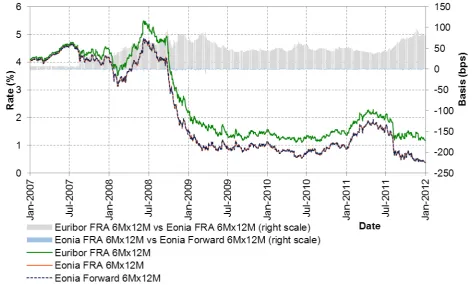
The above considerations, referred to spot rates, related to Deposit and OIS contracts, apply to forward rates as well, related to Forward Rate Agreement (FRA) contracts. In Figure 4 we show the historical series of quoted Euribor FRA 6Mx12M rates versus the quoted Eonia FRA 6Mx12M rates, versus the Euribor forward rate 6Mx12M implied by the two quoted Deposits on Euribor 6M and Euribor 12M.

The Euribor FRA 6Mx12M rate is the equilibrium (fair) rate of a FRA contract starting at spot date (today + 2 working days in the Euro market), maturing in 12 months, with a floating leg indexed to the Euribor 6M rate, versus a fixed interest rate leg. At maturity, the floating leg pays the interest accrued with the Euribor 6M rate fixed 6 months before, over the time interval [6M, 12M]. The fixed leg pays the interest accrued with the fixed rate, over the same time interval. Thus the FRA equilibrium rate reflects the market expectations over the future fixing of the underlying Euribor 6Mx12M rate.

The Eonia FRA is similar to the Euribor FRA, but the floating leg is indexed to Eonia, daily fixed and compounded over the time interval [6M, 12M].

The Euribor forward rate , referred to the generic time interval , is obtained through the standard formula (see e.g. Hull 2008),

spot rate is equivalent to discounting from to at the corresponding forward rate

and then discounting from to at the spot rate . Using equation 1, we compute the Euribor and Eonia forward rates as follows

(2)

(3)

where is the market rate quoted at time for an Euribor Deposit with maturity with tenor , is the market rate quoted at time for an Euribor FRA contract covering the period with tenor , is the Eonia OIS market rate quoted at time with maturity , is the market rate quoted at time for a Eonia FRA contract covering the interval and the subscript refers to the discount curve. In Figure 3 we depict the mechanism associated with the two equations 2 and 3 above.

Figure 3: the two figures describe the mechanism we implemented in order to replicate the FRA

market quotes.

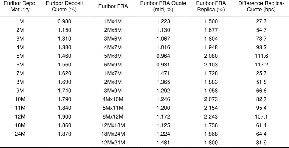
In Table 1 we report a snapshot of the numbers obtained on 30December 2011

Looking at the historical evolution in Figure 4, we observe that the three rates were essentially the same rate before the crisis, and diverged in August 2007, when the Forward, the Euribor FRA and the Eonia FRA acquired a positive basis with each other. The basis reached its maximum in

October 2008, in correspondence of the Lehman Brothers’ bankruptcy.

That difference can be justified by considering the nature of these rates. In particular, the credit an liquidity risk factors of FRA market equilibrium rates are mitigated by collateralization agreements that characterize FRA quoted contracts, while, in contrast, the deposit rates considered in the replication approach (i.e. Euribor Deposit 6M and Euribor Deposit 12M) are referred to unsecured transactions with different tenors (i.e. 6M and 12M) that, after the start of the crisis, reflect different liquidity and credit risk premia according to their maturity (Morini 2009).

Regarding the Eonia interest rate market, we compute the historical series of the Eonia Forward 6Mx12M rate during the interval Jan. 2007 – Dec. 2011 according to the equation 3 and we reported the results in Figure 5. We notice that the difference between the Eonia FRA 6Mx12M market rates and the corresponding forward rate is negligible over the whole observation period (average difference of 0.7 bps in absolute terms).

The Eonia OIS rates used for the FRA replica are obtained through the compounding of the Eonia O/N rate. Hence, the credit and liquidity risk components carried by the Eonia Forward rates can be considered negligible and consistent with the risk premia reflected by the Eonia FRA market rates.

In section 2.5 we report some findings of Mercurio (2009) who has proven that the above effects may be explained within a simple credit model that considers a default-free zero coupon bond and a risky zero coupon bond emitted by a defaultable counterparty.

t

1

Eonia FRA Replication (30 Dec. 2011)

Eonia OIS Maturity

Eonia OIS Quote (%)

Eonia FRA Start/End Dates

Eonia FRA Quote (%)

Eonia FRA Replica (%)

Difference Replica-Quote (bps)

1M 0.396 1Mx2M 0.392 0.392 0.0

2M 0.394 2Mx3M 0.386 0.385 -0.1 3M 0.391 1Mx4M 0.383 0.382 -0.1 4M 0.386 2Mx5M 0.371 0.370 -0.1

5M 0.380 3Mx6M 0.370 0.371 0.1

6M 0.381 6Mx12M 0.372 0.372 0.0 12M 0.376

Euribor FRA Replication (30Dec. 2011)

Euribor Depo. Maturity

Euribor Deposit

Quote (%) Euribor FRA

Euribor FRA Quote (mid, %)

Euribor FRA Replica (%)

Difference Replica-Quote (bps)

1M 0.980 1Mx4M 1.223 1.500 27.7 2M 1.150 2Mx5M 1.130 1.677 54.7 3M 1.310 3Mx6M 1.067 1.804 73.7 4M 1.380 4Mx7M 1.016 1.948 93.2 5M 1.460 5Mx8M 0.964 2.080 111.6 6M 1.560 6Mx9M 0.931 2.103 117.2 7M 1.620 1Mx7M 1.471 1.728 25.7 8M 1.690 2Mx8M 1.365 1.883 51.8 9M 1.740 3Mx9M 1.292 1.958 66.6 10M 1.790 4Mx10M 1.246 2.073 82.7 11M 1.840 5Mx11M 1.200 2.154 95.4 12M 1.900 6Mx12M 1.172 2.243 107.1 18M 1.860 12Mx18M 1.125 1.736 61.1 24M 1.870 18Mx24M 1.224 1.868 64.4 12Mx24M 1.481 1.800 31.9

Table 1: top panel: comparison between Eonia OIS, FRA and Forward rates for several start/end

Figure 4: Euribor FRA 6Mx12M market rate versus Eonia FRA 6Mx12M market rate versus Euribor Forward 6Mx12M rate (computed using equation 2). The corresponding spreads are shown on the right y-axis (Jan. 2007 – Dec. 2011 window, source: Bloomberg).

Figure 5: he Euribor FRA 6Mx12M market rate versus Eonia FRA 6Mx12M market rate versus

2.3. Basis Swaps

A third evidence of the regime change after the credit crunch is the explosion of the Basis Swaps spreads. In Figure 6 we report three historical series of quoted Basis Swap equilibrium spread, Euribor 3M vs Euribor 6M, Euribor 6M vs Euribor 12M, Euribor 3M vs Eonia, all at 5 years swap maturity. Basis Swaps are quoted on the Euro interbank market in terms of the difference between the fixed equilibrium swap rates of two swaps. For instance, the quoted Euribor 3M vs Euribor 6M Basis Swap rate is the difference between the equilibrium swap rates of a first standard swap with an Euribor 3M floating leg (quarterly frequency) vs a fixed leg (annual frequency), and of a second swap with an Euribor 6M floating leg (semi-annual frequency) vs a fixed leg (annual frequency).

The frequency of the floating legs is the “tenor” of the corresponding Euribor rates. The Eonia

floating legs are indexed to the shortest tenor rate (1 day), have annual frequency, and the floating coupon rate is given by the simple composition of the Eonia rates fixed daily during the coupon period.

As we can see in Figure 6, the Basis Swap spreads were negligible (or even not quoted) before the crisis. They suddenly diverged in August 2007 and peaked in October 2008 with the Lehman crash. Figure 7 reports spot Basis Swap spreads (reference date 30/12/2011) for different pairs of rates on several maturities. Basis Swap spreads not directly observable on the market have been computed from market quotations.

The Basis Swap involves a sequence of FRA rates carrying the credit and liquidity risk discussed in sections 2.1 and 2.2 above. Hence, the basis spread explosion can be interpreted in terms of the different credit and liquidity risk carried by the underlying FRA rates with different tenors, as in Figure 4. In Figure 6 and Figure 7 we see another example that, after the crisis, a swap floating leg indexed to the higher rate tenor (e.g. 6M) has an higher value with respect to the floating leg indexed to the shorter rate tenor (3M) with the same maturity, thus a positive spread emerges between the two corresponding equilibrium rates (or, in other words, a positive spread must be added to the 3M floating leg to equate the value of the 6M floating leg). In Figure 7 we observe that the magnitude of the Basis Swap spread increases with the tenor difference (see Bianchetti 2010 and Bianchetti 2011).

According to Morini (2009), a Basis Swap between two interbank counterparties under collateral agreement can be described as the difference between two investment strategies. Fixing, for instance, a Basis Swap Euribor 3M vs Euribor 6M with 6M maturity, scheduled on 3 dates ,

, , we have the following two strategies:

1. 6M floating leg: at choose a counterparty with an high credit standing (that is, belonging to the Euribor Contribution Panel) with collateral agreement in place, and lend the notional for 6 months at the Euribor 6M rate prevailing at (Euribor 6M flat because is an Euribor counterparty). At maturity recover notional plus interest from . Notice that if counterparty defaults within 6 months we gain full recovery thanks to the collateral agreement.

2. 3M+3M floating leg: at choose a counterparty with an high credit standing (belonging to the Euribor Contribution Panel) with collateral agreement in place, and lend the notional for 3 months at the Euribor 3M rate (flat) prevailing at . At recover notional plus interest and check the credit standing of : if has maintained its credit standing (it still belongs to the Euribor Contribution Panel), then lend the money again to for 3 months at the Euribor 3M rate (flat) prevailing at , otherwise choose another counterparty C2 belonging

to the Euribor Panel with collateral agreement in place, and lend the money to C2 at the

Figure 6: Basis Swap spreads: Euribor 3M Vs Euribor 6M, Euribor 6M Vs Euribor 12M and Eonia Vs Euribor 3M (Jan. 2007 – Dec. 2011 window, source: Bloomberg). All the quotations present a maturity of 5Y. Notice that the daily market quotations for some Basis Swap were not even available before the crisis.

Figure 7: Basis Swap spreads Eonia vs Euribor xM and Euribor xM vs yM over several maturities

Clearly, the 3M+3M leg implicitly embeds a bias towards the group of banks with the best credit standing, typically those belonging to the Euribor Contribution Panel. Hence, the credit risk carried by the 3M+3M leg must be lower than that carried by the 6M leg. In other words, the expected survival probability of the borrower in the 3M leg in the second 3M-6M period is higher than the survival probability of the borrower in the 6M leg in the same period. This lower risk is embedded into lower Euribor 3M + 3M rates with respect to Euribor 6M rates. But with collateralization the two legs have both negligible counterparty risk. Thus a positive spread must be added to the 3M+3M leg to reach equilibrium. The same discussion can be repeated, mutatis mutandis, in terms of liquidity risk.

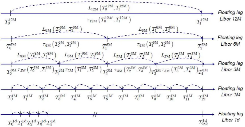
In Figure 8 we show a pictorial view of floating legs indexed to rates with different tenors. In equation 4 we report the corresponding leg values.

Figure 8: representation of floating Swap legs with different tenors (12M, 6M, 3M, 1M, 1d).

Before the financial crisis, since the liquidity and credit risk embedded in interbank rates with different tenors were very similar (and small), stream of cash flows with same maturity but different tenors could be replicated one with each others, and all these floating legs had the same value. The start of the financial turmoil and the consequent explosion of Basis Swap spread between rates with different tenors has invalidated classical no-arbitrage relations, such as equations 1 and 4, such that these floating legs acquired different values

where represents the net present value of the floating leg of a Swap indexed to the Euribor rate with tenor and with payment times according to the dates set

, is the FRA market rate referred to the period associated to the Euribor rate with tenor (i.e. ).

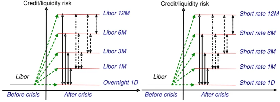
Figure 9: representation of the interest rate market segmentation.

We stress that the credit and liquidity risk involved here are those carried by the risky Libor rates underlying the Basis Swap, reflecting the average default and liquidity risk of the interbank money market (of the Libor panel banks), not those associated to the specific counterparties involved in the financial contract. We point out also that such effects were already present before the credit crunch, as discussed e.g. in Tuckman and Porfirio (2004), and well known to market players, but not effective due to negligible basis spreads.

𝐒𝐰𝐚𝐩12 , = , 12 12 , 12 12 , 12

≠ 𝐒𝐰𝐚𝐩6 , = , 𝑖 6 ,𝑖 6 𝑖 1, 𝑖 2

𝑖

≠ 𝐒𝐰𝐚𝐩3 , = , 𝑖 3 ,𝑖 3 𝑖 1, 𝑖 4

𝑖

≠ 𝐒𝐰𝐚𝐩1 , = , 𝑖 1 ,𝑖 1 𝑖 1, 𝑖 12

𝑖

≠ 𝐒𝐰𝐚𝐩1 , = , 𝑖 1 ,𝑖 1 𝑖 1, 𝑖 252

𝑖 ≠1 , _1𝑌

,𝑖 =

, _{𝑖 1}

, _𝑖 1 1

_𝑖 1, 𝑖

(4)

Short rate 12M

Short rate 6M

Short rate 3M

Short rate 1M

Short rate 1D

Libor

Before crisis After crisis Credit/liquidity risk Libor 12M

Libor 6M

Libor 3M

Libor 1M

Overnight 1D

Libor

Before crisis After crisis Credit/liquidity risk

2.4. The Credit and Liquidity Risk Components

In this section we try to highlight the credit and liquidity risk impact on the historical trend of the Euribor – Eonia basis during the period Jan. 2007 – Dec. 2011. To this aim, we introduce two different indexes that help us to underline credit and liquidity market stress periods.

Regarding the credit risk, we build an index representative of the credit risk in the European financial sector that we call Synthetic CDS Euribor Index. This index considers daily quotations of 5 years maturity CDS spread referred to financial institutions that belong to the Euribor panel in December 2011. Its computation replicates the fixing mechanism of the Euribor rates. Hence, for each reference date, we exclude the highest and the lowest 15% CDS spread quotations and compute the average of the remaining 70% quotes. The Synthetic CDS Euribor Index thus represents the average cost for protection against the default of a Libor panel bank within the European financial market.

Regarding the liquidity risk, we compute an index, called Liquidity Surplus Index, that considers official data reported by the ECB. The index is given by the sum of the total amount of the deposits posted by the EU financial institutions at the ECB’s Deposit Facility and of the current account holdings exceeding the EUR market-wide level minimum reserve requirement that are held by EU financial institutions at the ECB. We refer to this aggregation as a proxy of the liquidity surplus in the Euro zone interbank market.

The ECB requires credit and financial institutions to hold minimum reserves amounts on accounts managed by National Central Banks. The minimum reserve system has the scope of stabilizing the market interest rates and to facilitate the role of the ECB as liquidity supplier for the interbank market. The amount of minimum reserves is fixed, on a monthly basis, according to each financial

institution’s reserve base and the compliance of the requirements is verified considering the average, during a certain maintenance period, of the amounts posted at the reserve accounts. This mechanism ensures flexibility to financial institutions that can face minimum reserves provisions without compromising their business or investing opportunities. Holdings of required reserves are remunerated at the Main Refinancing Operation (MRO) rate, while holdings that exceeded the reserve requirement are free of remuneration. The minimum reserve is a liquidity absorption standing facility (ECB 2010).

The amounts posted by financial institutions at the Deposit Facility and the Excess Reserves help us to track liquidity stress of financial markets. Indeed, the higher is the Liquidity Surplus Index, the stronger is the preference to deposit cash reserves at the ECB instead of lending in the interbank market or investing in more profitable (and risky) activities.

In Figure 10 we report the historical series of the Synthetic CDS Euribor Index vs the Euribor 6M – Eonia OIS 6M basis, of the market quotes of the Basis Swap Eonia Vs Euribor 3M and of the Synthetic CDS Euribor Index over the period Jan. 2007 – Dec. 2011. We can observe that the Synthetic CDS Euribor Index reached a first peak in August 2007 in relation to the rise of concerns

over banks’ exposure to credit structured products (i.e. CDO, ABS etc.). This first increase of the

premia against the default of primary financial institutions matched the explosion of the Euribor – Eonia basis (Figure 10 – spot 1) and it highlights a generalized growth of the default risk perceived in the interbank market reflected by an increase of the Euribor rates (see Figure 1).

correspondence of Italy’s credit rating cut, and it was very far from the pre-crisis level when banks

where considered “too big to fail”. This rise in the credit risk was matched by an increase of the

Euribor – Eonia basis that reached 127 bps on 01December 2011 (Figure 10 – spot 6).

Figure 10: Synthetic CDS Euribor Index 5Y spread (line), Basis Swap Eonia Vs Euribor 3M 5Y

spread (line, right scale) and Euribor Deposit 6M – Eonia OIS 6M basis (area) from Figure 1 (Jan. 2007 – Dec. 2011 window, sources: Bloomberg and ICAP). Notice that the basis swap has the same payment frequency (3 months) and maturity (5Y) of the Synthetic CDS Index.

Regarding the relation between the Basis Swap Eonia Vs Euribor 3M and the Synthetic CDS Euribor Index, we can observe a close trend of the two historical series, especially in correspondence of an increase of the credit risk perceived in the interbank market. The increase of the Basis Swap spread in correspondence of a rise in the average default risk seems to reveal a stronger relevance of the credit risk component over longer maturities (i.e. 5Y).

The liquidity risk component in Euribor and Eonia interbank rates is distinct but strongly related to the credit risk component. According to Acerbi and Scandolo (2007), liquidity risk may appear in at least three circumstances:

1. lack of liquidity to cover short term debt obligations (funding liquidity risk),

2. difficulty to liquidate assets on the market due excessive bid-offer spreads (market liquidity risk),

3. difficulty to borrow funds on the market due to excessive funding cost (systemic liquidity risk).

Following Morini (2009), these three elements are, in principle, not a problem until they do not appear together, because a bank with, for instance, problem 1 and 2 (or 3) will be able to finance itself by borrowing funds (or liquidating assets) on the market. During the crisis these three scenarios manifested themselves jointly at the same time, thus generating a systemic lack of liquidity (see e.g. Michaud and Upper 2008).

0 10 20 30 40 50 60 70 80 0 50 100 150 200 250 300 350 400 J a n -2007 J u l-2007 J a n -2008 J u l-2008 J a n -2009 J u l-2009 J a n -2010 J u l-2010 J a n -2011 J u l-2011 J a n -2012 B a s is S w a p S p re a d ( b p s ) S p re a d ( b p s ) Date Euribor Deposit 6M - Eonia OIS 6M Basis Synthetic CDS Euribor Index 5Y Spread

Basis Swap Eonia vs Euribor 3M 5Y Spread (right scale)

Clearly, it is difficult to disentangle liquidity and credit risk components in the Euribor and Eonia rates, because, in particular, they do not refer to the default risk of one counterparty in a single derivative deal but to a money market with bilateral credit risk (see the discussion in Morini (2009) and references therein).

In the Euro system the ECB is responsible of ensuring and maintaining the liquidity of the financial market through several monetary facilities and open market operations. Any liquidity injection in the interbank market should be absorbed by financial institutions. Before the financial turmoil, the

liquidity provided by the ECB aimed mainly to satisfy the market’s liquidity needs and banks could

rely on an easy and convenient access to the interbank market for their short term liquidity operations.

In Figure 11 we compare the historical trend of the Synthetic CDS Euribor Index, of the Liquidity Surplus Index, of the Euribor 6M – Eonia OIS 6M basis and of the Basis Swap Eonia Vs Euribor 3M. The first main intervention of the ECB during the financial crisis was in October 2008 (Figure 11 – spot 1) an it regarded the adoption of several measures such as the cut of the official interests rates in conjunction with others central banks3_{, the introduction of a fixed-rate refinancing operation}

with full-allotment, the extension of the securities accepted as collateral by the central bank and the increase of the number of financial institutions that can accede to the ECB monetary policy channels (ECB 2008a, 2008b, 2008c, 2008d). As we can observe in Figure 11, the new monetary policy decisions put in force by the ECB led to a sudden explosion of the Liquidity Surplus that exactly matches the most relevant increase experienced by the Euribor – Eonia spread during the period Jan. 2007 – Dec. 2011.

The Liquidity Surplus Index reached a second peak on the 25June 2009 (Figure 11 – spot 2) and its increase is due to the introduction by the central bank of a LTRO with a 12M term (ECB 2009a). This non-standard facility provided the European financial market with an unlimited amount of liquidity with 1 year maturity. This intervention reduced the liquidity shortage of the market and it is accompanied by a reduction of the Euribor – Eonia basis and a decrease of the credit risk reflected by the Synthetic CDS Euribor Index.

At the end of the 2009 (Figure 11 – spot 3) we can notice a third jump in the liquidity amount posted at the ECB. This sudden variation can be ascribed to the extension of the fixed-rate refinancing operations with full allotment introduced in October 2008 (ECB 2009b).

From Figure 11 we note that the Liquidity Surplus index experienced an upward trend during the period Jan. 2010 – Jul. 2010 that is exacerbated in May 2010 by the worsening of the so called

“sovereign debt crisis” related to market concerns over Greece’s capability to maintain its debt obligations. The effects of this market uncertainty are reflected also by the Synthetic CDS Euribor index that increased almost up to 200 bps in June 2010. The LTRO introduced in June 2009 by the ECB expired at the end of May 2010 (Figure 11 – spot 4). The amount of liquidity surplus shrank significantly and the Liquidity Surplus Index decreased until July 2011.

During the period Jul. 2009 – Jul 2011 the Euribor – Eonia basis has maintained a relative stable and low level compared to Aug. 2007 – Jun. 2009, showing contained peaks in correspondence of a simultaneous increase of both the Liquidity Surplus Index and the Synthetic Surplus Index. The second half of the 2011 was characterized by the second phase of the sovereign debt crisis that started to affect countries such as Italy and Spain. The market conditions in terms of credit and liquidity risk deteriorated significantly and that was promptly reflected by the increase of both the Liquidity Surplus Index and the Synthetic CDS Euribor Index. In this period the Eonia OIS rates decreased significantly and Euribor rates remained almost stable (see Figure 1) leading to a relevant rise of the correspondent basis.

The Liquidity Surplus Index reached its maximum on the 22nd December 2011 (Figure 11 – spot 5)

in correspondence of the ECB’s decision to put in place a multi-tranche LTRO with a maturity of 3 years (ECB 2011). The first LTRO tranche, which took place in the 21December 2011, provided

value of €483 billion and almost all the liquidity offered to the market by the ECB was posted at the

ECB’s accounts. The difficult credit and liquidity conditions experienced by the European financial market in the last half of 2011 led to a significant increase in the Euribor – Eonia basis.

Figure 11: Synthetic CDS Euribor index 5Y (line), Liquidity Surplus Index of the European

interbank market (line, right scale), Basis Swap Eonia Vs Euribor 3M 5Y (line) and Euribor Deposit 6M – Eonia OIS 6M basis (area). We multiplied by 4 the Basis Swap Eonia Vs Euribor 3M 5Y to better compare its historical trend (window Jan. 2007 – Dec. 2011, sources: Bloomberg and ECB).

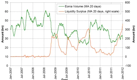
In Figure 12 we compare the trend of the Liquidity Surplus index and of the Eonia Volume. We can observe that an increase in the liquidity amount posted at the ECB is always accompanied by a reduction of the total amount traded in the European money market. The drain of liquidity that affected the money market is the main reason of the closeness of the Eonia rate to the Deposit Facility rate during the financial crisis (see Figure 2).

By considering the trend of the Liquidity Surplus Index we argue that from the Lehman Brothers’

bankruptcy up to the end of the 2011 the liquidity risk factor has played a key role, in conjunction with the credit risk, in explaining the trend of the Euribor – Eonia basis. Generally, we can observe an increase of the difference between Euribor and Eonia OIS rates when both the Synthetic CDS Euribor Index and the Liquidity surplus Index start to go up. This combined upward movement reveals an increase of the overall risk perceived within the interbank market. Observing the historical series reported in Figure 11, we claim that the Euribor – Eonia basis’ peak of October 2008 is caused, initially, by the increase in the average default risk of the market in correspondence of the Lehman crash and, subsequently, by the liquidity risk in the interbank market and the drastic official interest rate cut operated by the ECB during that period. Also in the second half of 2011, the upward trend of the Euribor – Eonia basis was driven by a simultaneous rise of both the credit and liquidity risk in the interbank market, reflected in the market through a decrease of the Eonia OIS rates and almost stable Euribor rates.

-100 0 100 200 300 400 500 600 0 50 100 150 200 250 300 350 400 J a n -2007 J u l-2007 J a n -2008 J u l-2008 J a n -2009 J u l-2009 J a n -2010 J u l-2010 J a n -2011 J u l-2011 J a n -2012 A m o u n t (b n ) S p re a d ( b p s ) Date

Euribor Deposit 6M - Eonia OIS 6M Basis Basis Swap Eonia vs Euribor 3M 5Y Spread (x4) Synthetic CDS Euribor Index 5Y

Liquidity Surplus Index (right scale)

1 2

3

4

Figure 12: moving average 20 days of the Liquidity Surplus index and of the Eonia Volume (window Jan. 2007 – Dec. 2011). Note that we reported the Eonia Volume on the right scale since the two historical series present different magnitudes. (Sources: Bloomberg, ECB).

2.5. A Simple Credit Model

In order to explain the basis divergence after the credit crunch, Mercurio (2009) proposed a simple credit model, including the default risk relative to an average interbank counterparty

We assume that the risky Libor rate fixed on the interbank market by the Libor panel is precisely the funding rate over the time interval of an abstract “average” Libor Bank. We may define as usual a discount factor such that

(5)

(6)

where , is the value in of a default free zero coupon bond with maturity , is the expected value in under the risk neutral probability measure , is the default free instantaneous interest rate, and , are the spot and forward default probabilities of the Libor Bank, respectively. By considering the above assumptions, the risky Libor rate is given by

₍₇₎

Using equation 7 above, we can obtain the price in of a standard FRA contract that exchanges in the fixed rate versus the risky Libor rate as

(8)

where is the notional of the contract, for a payer/receiver FRA (referred to the fixed leg). The price of the market FRA is obtained through an analogous proof as

We stress that the prices in equations 8 and 9 above have been nder the assumption that the FRA contract (not the underlying Libor rate) is credit risk free. Otherwise the derivation would involve the default indicator of the two counterparties involved in the FRA contract (not that of the average Libor Bank).

Assuming that the FRA contract is in equilibrium, such that , denoting with _{the equilibrium FRA rate at time and rearranging equations 8 and 9, we obtain}

₍₁₀₎

Since and , we have that then

(11)

where is the default free forward rate. We conclude that, thanks to default risk, the risky FRA rate is always higher than the corresponding forward rate relative to a default free yield curve. In other words, the default risk of the average Libor Bank, included into the Libor rate underlying a risk free FRA contract, induces a positive basis spread between the equilibrium FRA rate and a corresponding risk free forward rate. Only in the special case of a risk free Libor Bank, such that

, we have

(12)

A risk free derivative could sound a little strange, in a market where even Libor Banks may default, but actually this ideal condition can be approximated in practice using collateralization, as discussed in the next section.

3. Collateralization and CSA Discounting

Another effect of the credit crunch has been the great diffusion of collateral agreements to reduce the counterparty risk of OTC derivatives positions. In the following sections we discuss some of the relevant aspects that concern the collateralization process.

3.1. Collateral Diffusion

Figure 13: growth of the collateral value over the last 12 years (source: ISDA 2012a).

respondents that present active collateral agreements between 3000 and 100 are classified as medium market participant. Small dealers are financial institution and companies that report less than 100 active contracts. Among the 51 respondents, 14 are classified as large dealers and belong to the financial sector. The total number of respondents to the Margin Survey in 2012 is 51. Figure 13 shows the growth in value of reported and estimated collateral in circulation within the OTC derivatives market. We can observe an upward trend of the collateral value over all the past 12 years, except between 2008 and 2010 where the reduction can be ascribed to a decrease in the market activity. During the 2011 the reported and the estimated value of collateral have experienced an increase of 24%.

As shown in Table 2, more than 80% of all OTC derivatives are collateralized among large dealers. Credit derivative contracts present the highest frequency of collateralization followed by Fixed Income derivatives. The FX derivatives show the lowest percentage of collateralization (58.3%), but their poor result can be explained by the fact that this type of contract is usually characterized by short maturities that, compared to the other contract classes, help to mitigate the counterparty risk. The percentages of collateralization related to large dealers are always higher than those of other classes of market participants, regardless the type of OTC Derivatives.

All Large Dealers

All OTC Derivatives 71.4% 83.7%

Fixed Income Derivatives 78.1% 89.9%

Credit Derivatives 93.4% 96.1%

FX Derivatives 55.6% 70.6%

Equity Derivatives 72.7% 85.3%

Commodities Derivatives 56.3% 63.9%

Table 2: percentage of trades subjected to collateral agreements by derivative and dealer type

3.2. Collateral Mechanics

A typical financial transaction generates streams of future cash flows whose total net present value (NPV) is the algebraic sum of all discounted expected cash flows. Generally, each transaction implies a mutual credit exposure between two counterparties, let’s say, a bank ( ) and a generic market counterparty ( ). If, at any time during the life of the transaction, for counterparty we have that , then counterparty expects to receive, on average, future cash flows from counterparty (in other words, has an expected credit with at time ). On the other side, if counterparty has , then it expects to pay, on average, future cash flows to counterparty (in other words, has an expected debt with at time ). The reverse holds if

and .

Such credit/debit exposure is clearly subject to bilateral default risk, the probability that the debtor counterparty may default, not fulfilling its obligations with the creditor counterparty. This credit risk

can be mitigated through a guarantee, called “collateral agreement”. This guarantee is formalised

into an optional annex of the ISDA Master Agreement (the standard legal contract widely used to regulate OTC transactions) called Credit Support Annex (CSA). The main feature of the CSA is the additional obligation of the counterparties for a margination mechanism similar to those adopted by Central Counterparties (CCPs, i.e. LCH.Clearnet, Euroclear, SIX Securities Services, etc.) for OTC derivatives clearing, or by exchanges for standard market instruments clearing (i.e. Futures). In a nutshell, at every margination date the two counterparties check the value of the portfolio of mutual OTC transactions and regulate the margin, adding to or subtracting from the collateral account the corresponding mark to market variation with respect to the preceding margination date. The margination can be regulated with cash or with (primary) assets of corresponding value. In any case the collateral account holds, at each date, the total NPV of the portfolio, which is positive for the creditor counterparty and negative for the debtor counterparty. The collateral amount is available to the creditor.

On the other side, the debtor receives an interest on the collateral amount, called “collateral rate”. Hence, we can look at the CSA as a funding mechanism, transferring liquidity from the debtor to the creditor. The main differences with traditional funding through Deposit contracts are that, using derivatives, we have longer maturities and variable (stochastic) lending/borrowing sides and amounts. We can also look at CSA as an hedging mechanism, where the collateral amount hedges the creditor against the event of default of the debtor. The most diffused CSA provides a daily margination mechanism and an overnight collateral rate (ISDA 2012a). Actual CSAs provide many other detailed features (i.e. credit support amount, delivery amount, minimum transfer amount, collateral currency, etc.) that are out of the scope of the present discussion.

Figure 14 illustrates a general scheme of funding with or without CSA that we briefly introduced above. When both the counterparties can post and receive collateral, the CSA mechanisms is

3.3. CSA Discounting

A first important consequence of the diffusion of collateral agreements among interbank

counterparties is that we can consider the derivatives’ prices quoted on the OTC interbank market as transactions between counterparties under CSA. A second important consequence is that, by no-arbitrage and self-financing conditions, the CSA margination rate and the discounting rate of

future cash flows must match, hence the name of “CSA discounting” (or “OIS discounting”). In

particular, the most diffused overnight CSA implies overnight-based discounting and the construction of a discounting yield curve that must reflect, for each maturity, the funding level in an overnight collateralized interbank market. Thus OIS are the natural instruments for the discounting curve construction, that are also the best available proxies of risk free rates (see Ametrano and Bianchetti 2009, Bianchetti 2010).

The CSA discounting approach for the evaluation of collateralized OTC trades can be described by considering a simple cash flow transaction trade between two generic default free counterparties (bank and a generic market counterparty ) with payoff at maturity time . We assume that the deal is under perfect collateralization with margination dates , where

, and perfect collateral account such that

for each ,

,

where is the simply compounded collateral rate (i.e. Eonia) fixed at time and covering the interval . The payoff of the trade and the structure of the margination dates are shown in Figure 15.

Figure 14: two-way-CSA with cash collateral and no-CSA funding mechanics.

Bank Two-Way-CSA

Collateral And Funding

Desk

Trading Desk

Money Market Counterparty Market

Counterparty

Collateral Amount

received/posted under CSA

interest paid/received on

under CSA

𝑖

interest paid/received on

without CSA

Borrowing/Lending amount without

CSA

Lending/Borrowing at

Figure 15: simple deal with a single cash flow payoff and multiple margination dates.

Suppose that the trade is under collateral with only two margination dates, and , and receives a positive amount at maturity , which correspond to a present value at time

, as depicted in Figure 16. Hence, counterparty posts an amount into the collateral bank account that grows at the collateral rate up to maturity . By no-arbitrage and self-financing we have

where

We can conclude that, by simple no-arbitrage arguments, future cash flows associated with collateralized trades must be discounted at the collateral rate.

Figure 16: trade and collateral account cash flows scheme.

In case of absence of CSA, using the same no-arbitrage and self-financing principles between the funding and the discounting rate, we argue that future cash flows (positive or negative) must be discounted using the corresponding funding term structure. This implies important (and rather involved) consequences, such that, according with Morini and Prampolini (2011), each counterparty assigns a different present value to the same future cash flow, breaking the fair value symmetry. Indeed, a worsening of the its credit standing allows the Bank to sell derivatives (options in particular) at more competitive prices (the lower the rate, the higher the discount, the lower the price).

We stress that before the crisis the old-style standard Libor curve was representative of the average funding level on the interbank market (see e.g. Hull 2008). Such curve, even if considered a good proxy for a risk free curve, due to the perceived low counterparty risk of primary banks (belonging to the Libor Contribution panel), was not strictly risk free because of the absence of collateralization.

CSA are reduced. The new SCSA introduces different “silos” corresponding to the currencies with the most liquid OIS curves (e.g. EUR, USD, GBP, CHF, JPY). Each transaction is allocated to one single silo, in relation with the currency of the underlying, with the relevant OIS rate used to

discount all the trade’s cash flows. According to this mechanics, counterparties will have to manage multiple flows of collateral in different currencies that will create a systemic cross currency settlement risk (i.e. two counterparties, two swaps, one in EUR, one in USD). To solve the problem the SCSA allows counterparties to net collateral flows denominated in multiple currencies into a single payment in a single currency using the overnight currency swap market to exchange the flows (ISDA 2012b). However, implementing the SCSA requires to solve some relevant challenges such as the adoption of a common set of exchange rates and calculation specifications for managing collateralized trades.

3.4. Market Quotes

During the financial crisis, the market has experienced a transitional phase from the classical Libor-based discounting methodology to the modern CSA Libor-based discounting methodology. As we notice in section 3.1, OTC transactions executed on the interbank market normally use CSA discounting. In particular, plain vanilla interest rate derivatives, such as FRA, Swaps, Basis Swaps, Caps/Floor/Swaptions are quoted by main brokers using CSA discounting.

In particular in September 2010 the international broker ICAP switched to OIS discounting, publishing both Libor- and OIS-based cap/floor/swaption implied volatilities. Since January 2012 only OIS-based volatilities are published (ICAP 2010, 2011).

Figure 17: EUR at-the-money Swaption market quotes on 30June 2010. Premia (left panel) and

Black’s implied volatilities (right panel). The ATM implied volatilities surface is obtained using the classical single-curve approach. (Source: ICAP).

Figure 18: EUR at-the-money Swaption market quotes on 30 September 2010. Premia are

distinguished between spot (panel A) and forward ones (panel C). Implied spot premia are obtained from forward premia using Eonia discounting. Implied volatilities quotes are now differentiated between the Euribor one (panel B) and the Eonia one (panel D). (Source: ICAP).

A B

Option Expiry 1Y 2Y 3Y 4Y 5Y 6Y 7Y 8Y 9Y 10Y 15Y 20Y 25Y 30Y Option Expiry 1Y 2Y 3Y 4Y 5Y 6Y 7Y 8Y 9Y 10Y 15Y 20Y 25Y 30Y 1M Opt 11 24.5 38.5 53 68 83.5 99 115 129 144 205 261 319 389 1M Opt 46.4 39.2 35.9 32.3 29.9 28.1 27 26.3 25.6 25.1 23.3 23.5 24.9 27.6 2M Opt 16.5 37 58 79.5 101 122 143 163 183 203 290 373 456 548 2M Opt 48.8 40.6 37 33.4 30.8 28.6 27.1 25.9 25.2 24.7 23.1 23.5 25 27.3 3M Opt 22.5 50.5 77.5 104 129 153 177 201 225 250 355 458 564 666 3M Opt 51.7 44.1 39.5 34.8 31.2 28.7 27 25.8 25 24.6 22.9 23.4 25.1 27 6M Opt 37.5 81 121 158 195 231 265 298 330 362 499 624 763 919 6M Opt 57.9 47.4 41.2 35.9 32.2 29.7 27.8 26.5 25.5 24.8 22.7 22.6 24.1 26.4 9M Opt 50 107 157 205 252 295 337 378 417 455 622 767 931 1104 9M Opt 59.9 48.4 41.4 36.2 32.7 30.1 28.2 26.9 25.9 25.1 22.9 22.6 24 26 1Y Opt 61.5 126 186 245 300 352 402 449 495 536 734 900 1081 1256 1Y Opt 59.5 46.6 40.2 35.7 32.4 30 28.3 27.1 26.1 25.1 23.2 22.9 24.1 25.6 18M Opt 78.5 158 233 305 373 437 498 557 612 666 902 1116 1318 1512 18M Opt 53.9 42.1 36.9 33.2 30.6 28.7 27.4 26.3 25.4 24.8 23 23.1 24 25.2 2Y Opt 94 183 268 349 427 503 574 641 705 767 1028 1259 1492 1708 2Y Opt 48.2 37.6 33.5 30.6 28.6 27.3 26.3 25.4 24.6 24.1 22.5 22.5 23.6 24.7 3Y Opt 111 214 312 405 494 581 663 740 815 888 1182 1447 1726 1991 3Y Opt 35.5 29.9 27.4 25.8 24.7 24 23.3 22.8 22.3 22 20.9 21.2 22.5 23.8 4Y Opt 121.5 235 341 441 537 630 719 803 885 965 1282 1571 1874 2153 4Y Opt 28.3 25.2 23.8 22.9 22.2 21.7 21.2 20.9 20.6 20.5 19.8 20.3 21.6 22.8 5Y Opt 126.5 244 357 464 565 661 754 842 929 1011 1351 1656 1963 2274 5Y Opt 24 22.1 21.5 21 20.5 20.1 19.8 19.6 19.4 19.4 19.1 19.7 21 22.3 7Y Opt 129 250 367 480 587 686 783 878 971 1062 1411 1730 2049 2375 7Y Opt 19.7 19 18.8 18.5 18.3 18.1 18 18 18 18.2 18.2 19 20.2 21.4 10Y Opt 128.5 247 364 477 586 689 791 891 988 1082 1444 1763 2092 2404 10Y Opt 16.9 16.5 16.5 16.6 16.8 16.9 17 17.2 17.5 17.7 18.2 19.1 20.2 21.2 15Y Opt 123 235 348 461 569 673 775 874 968 1057 1407 1722 2043 2352 15Y Opt 17 16.9 17.2 17.6 18.1 18.5 18.8 19.3 19.7 20 20.7 21.3 22 22.6 20Y Opt 113.5 220 326 434 540 640 736 829 915 994 1337 1627 1910 2164 20Y Opt 19.9 20.2 20.8 21.8 22.6 23.2 23.8 24.3 24.6 24.7 24.4 23.8 23.6 23.3 25Y Opt 104.5 201 300 401 500 591 676 764 843 918 1220 1483 1726 1946 25Y Opt 26 26.1 26.8 27.8 28.5 28.6 28.4 28.4 28 27.7 25.3 23.7 22.7 22.4 30Y Opt 95 180 267 355 442 522 598 676 746 812 1092 1337 1569 1791 30Y Opt 27.6 26.2 26 26 26.1 25.8 25.5 25.4 25 24.6 22.4 21.1 20.8 21.2

Sw ap Tenor Maturity

30/06/2010 - EUR ATM Sw aption Straddles - Prem ium Mids 30/06/2010 - EUR ATM Sw aption Straddles - Im plied Volatilities

A B

Option Expiry 1Y 2Y 3Y 4Y 5Y 6Y 7Y 8Y 9Y 10Y 15Y 20Y 25Y 30Y Option Expiry 1Y 2Y 3Y 4Y 5Y 6Y 7Y 8Y 9Y 10Y 15Y 20Y 25Y 30Y 1M Opt 10.5 25.5 41 57.5 76.5 96.5 117 138 161 185 270 346 420 494 1M Opt 40.5 38.4 37.9 36.8 36.4 35.9 35.5 35.4 35.8 36.4 34.4 34.4 36.1 38.6 2M Opt 15.5 37.5 60 85.5 115 141 168 198 227 261 379 486 592 700 2M Opt 40.4 38.6 37.6 37.2 37.1 35.8 34.9 34.7 34.6 35.1 33.2 33.3 35 37.7 3M Opt 20 49.5 78.5 110 142 176 209 243 278 315 458 583 711 841 3M Opt 41.1 40.8 39.5 38.4 37.2 36.1 35.1 34.6 34.4 34.5 32.8 32.7 34.5 37.1 6M Opt 32 76.5 116 159 205 250 293 340 385 430 620 796 961 1131 6M Opt 44.1 42.8 39.8 38.1 36.8 35.3 34.2 33.7 33.2 32.9 31.2 31.6 33 35.4 9M Opt 44.5 98.5 149 202 255 308 361 414 468 523 751 953 1148 1358 9M Opt 47 43.1 40.3 38 36.1 34.6 33.5 32.8 32.4 32.1 30.6 30.7 32.1 34.6 1Y Opt 54.5 117 177 235 296 360 419 479 540 599 852 1074 1300 1526 1Y Opt 47.6 42.7 39.7 37 35.2 34.1 33 32.3 31.8 31.4 29.9 29.9 31.5 33.7 18M Opt 75 149 222 296 369 441 512 582 655 729 1020 1286 1542 1792 18M Opt 48.8 41.2 38.1 35.8 34 32.7 31.8 31.1 30.7 30.5 29 29.2 30.6 32.5 2Y Opt 92.5 179 262 344 428 510 589 667 747 825 1156 1449 1731 2002 2Y Opt 47.8 40.1 36.7 34.1 32.6 31.5 30.7 30 29.6 29.3 28.2 28.5 29.9 31.6 3Y Opt 112.5 217 315 411 509 604 697 785 874 967 1328 1665 1992 2305 3Y Opt 40.8 35 32.2 30.4 29.5 28.7 28.2 27.6 27.3 27.3 26.3 26.9 28.5 30.2 4Y Opt 124.5 240 349 455 556 658 756 852 946 1049 1427 1778 2125 2447 4Y Opt 34.3 30.3 28.5 27.4 26.6 26.1 25.6 25.3 25.1 25.3 24.5 25.3 26.9 28.4 5Y Opt 131 253 367 476 583 689 792 895 996 1100 1497 1852 2197 2549 5Y Opt 29.2 26.7 25.6 24.8 24.3 24 23.7 23.6 23.6 23.8 23.4 24.1 25.6 27.2 7Y Opt 133.5 259 377 494 606 717 825 928 1031 1141 1539 1900 2249 2605 7Y Opt 23.6 22.5 22 21.6 21.3 21.2 21.3 21.3 21.4 21.7 21.6 22.6 23.9 25.4 10Y Opt 136 263 388 508 626 739 849 953 1058 1166 1563 1928 2270 2594 10Y Opt 20 19.5 19.6 19.7 19.8 19.9 20 20.1 20.3 20.6 21.1 22.3 23.4 24.3 15Y Opt 130 251 371 487 598 709 817 922 1029 1134 1515 1888 2223 2539 15Y Opt 19.3 19.2 19.4 19.6 19.8 20.2 20.7 21.2 21.7 22.3 23.3 24.4 25.1 25.4 20Y Opt 119.5 235 348 460 569 676 780 881 981 1068 1444 1780 2087 2356 20Y Opt 21.4 22.1 22.9 23.7 24.5 25.3 26.1 26.8 27.4 27.7 27.8 27.5 27 26.3 25Y Opt 110 214 320 426 528 628 722 811 904 990 1324 1621 1896 2142 25Y Opt 28.2 29.3 30.3 31.4 32.1 32.6 32.6 32.5 32.6 32.3 29.6 27.5 26.1 25.5 30Y Opt 101.5 196 289 384 477 565 651 732 816 893 1203 1485 1751 2012 30Y Opt 32.5 31.5 31.1 31.1 31.1 30.9 30.7 30.3 30.1 29.6 26.2 24.4 23.9 24.4

C D

Option Expiry 1Y 2Y 3Y 4Y 5Y 6Y 7Y 8Y 9Y 10Y 15Y 20Y 25Y 30Y Option Expiry 1Y 2Y 3Y 4Y 5Y 6Y 7Y 8Y 9Y 10Y 15Y 20Y 25Y 30Y 1M Opt 10.5 25.5 41 57.5 76.5 96.5 117 138 161 185 270 346 421 495 1M Opt 40.6 38.4 37.9 36.8 36.3 35.8 35.5 35.4 35.8 36.4 34.4 34.4 36.1 38.6 2M Opt 15.5 37.5 60 86 115 141 169 198 228 261 379 486 592 701 2M Opt 40.4 38.6 37.6 37.1 37.1 35.8 34.9 34.7 34.6 35.1 33.2 33.3 35 37.7 3M Opt 20 49.5 78.5 110 142 176 209 243 278 315 459 584 712 842 3M Opt 41.1 40.8 39.5 38.3 37.1 36.1 35.1 34.6 34.4 34.5 32.8 32.7 34.4 37 SM Opt 32 76.5 116 160 206 250 294 341 386 431 622 799 964 1135 6M Opt 44.1 42.7 39.7 38 36.7 35.3 34.1 33.6 33.1 32.8 31.2 31.5 33 35.3 9M Opt 44.5 99 150 203 257 310 363 417 471 526 756 959 1155 1366 9M Opt 46.9 43 40.2 37.8 36 34.5 33.4 32.7 32.3 32.1 30.6 30.6 32.1 34.5 1Y Opt 55 118 178 237 299 363 423 483 545 605 859 1083 1311 1539 1Y Opt 47.5 42.5 39.6 36.8 35.1 34 32.9 32.2 31.7 31.3 29.8 29.8 31.4 33.6 18M Opt 76 151 225 300 374 447 519 590 664 739 1035 1303 1564 1817 18M Opt 48.7 41 37.9 35.6 33.8 32.5 31.6 30.9 30.5 30.3 28.8 29 30.5 32.3 2Y Opt 94.5 183 268 351 437 520 601 681 762 842 1179 1479 1767 2042 2Y Opt 47.6 39.8 36.4 33.8 32.4 31.3 30.5 29.8 29.4 29.1 28 28.3 29.7 31.4 3Y 0pt 116.5 225 327 426 528 625 722 814 906 1002 1376 1726 2064 2388 3Y Opt 40.5 34.6 31.9 30 29.2 28.4 27.9 27.4 27 27 26 26.6 28.2 29.8 4Y 0pt 131.5 254 369 480 588 695 798 900 999 1108 1507 1878 2244 2585 4Y Opt 34 29.9 28.1 27 26.2 25.7 25.3 25 24.8 24.9 24.2 24.9 26.5 27.9 5Y 0pt 141.5 273 396 514 630 744 856 967 1076 1189 1618 2001 2374 2754 5Y Opt 28.9 26.3 25.2 24.4 23.9 23.6 23.3 23.2 23.2 23.4 23 23.7 25.1 26.7 TY 0pt 152 295 431 564 691 819 942 1059 1177 1302 1757 2168 2567 2974 TY Opt 23.2 22 21.5 21.1 20.8 20.8 20.8 20.8 20.9 21.2 21.1 22 23.3 24.7 10Y 0pt 170.5 329 487 638 785 927 1065 1195 1327 1463 1960 2419 2848 3255 10Y Opt 19.6 18.9 19 19.1 19.2 19.3 19.4 19.5 19.7 20 20.4 21.6 22.6 23.5 15Y 0pt 193 374 552 725 890 1055 1217 1373 1532 1688 2256 2810 3309 3780 15Y Opt 18.8 18.4 18.6 18.8 19 19.4 19.8 20.3 20.8 21.4 22.2 23.3 23.9 24.2 20Y 0pt 209 410 608 804 994 1181 1363 1539 1714 1866 2523 3110 3645 4115 20Y Opt 20.6 20.9 21.6 22.4 23.1 23.9 24.5 25.2 25.8 26 26 25.8 25.2 24.7 25Y 0pt 218 424 633 843 1047 1244 1430 1607 1791 1961 2622 3209 3755 4241 25Y Opt 27.2 27 28.1 29 29.4 29.6 29.4 29.2 29.3 29.6 27.2 25.3 24.1 23.7 30Y 0pt 220.5 425 629 833 1035 1227 1414 1590 1771 1939 2613 3226 3803 4369 30Y Opt 29.2 26.9 26.7 26.9 28 27.1 27.2 27 27.1 26.8 23.9 22.3 22 22.3

Sw ap Tenor

Sw ap Tenor Sw ap Tenor

Sw ap Tenor