N Rotating Loop Soliton Solution of the Coupled Integrable Dispersionless Equation

(1)

ISSN Online: 2327-4379 ISSN Print: 2327-4352

N-Rotating Loop-Soliton Solution of the

Coupled Integrable Dispersionless Equation

Souleymanou Abbagari

1,2,3,4

, Saliou Youssoufa

2,3,4

, Hermann T. Tchokouansi

2,3,4

,

Victor K. Kuetche

2,3,4

_{, Thomas B. Bouetou}

2,3,4

_{, Timoleon C. Kofane}

2,4

1_{Department of Basic Science, Law and Humanities, Institute of Mines and Petroleum Industries, University of Maroua,}

Maroua, Cameroon

2_{Laboratory of Mechanics, Materials and Structures, Department of Physics, University of Yaoundé I, Yaoundé, Cameroon}

3_{National Advanced School of Engineering, University of Yaoundé I, Yaoundé, Cameroon}

4_{Centre d’Excellence en Technologies de l’Information et de la Communication (CETIC), University of Yaoundé I,}

Yaoundé, Cameroon

Abstract

In this paper, we investigate the Rotating N Loop-Soliton solution of the coupled integrable dispersionless equation (CIDE) that describes a current-fed string within an external magnetic field in 2D-space. Through a set of inde-pendent variable transformation, we derive the bilinear form of the CIDE Eq-uation. Based on the Hirota’s method, Perturbation technique and Symbolic computation, we present the analytic N-rotating loop soliton solution and proceed to some illustrations by presenting the cases of three- and four-soliton solutions.

Keywords

Coupled Integrable Dispersionless Equation, Bilinear Method, Soliton Solutions, Perturbation Technique, Symbolic Computation

1. Introduction

During the past several years, the study of coupled nonlinear evolution Equa-tions has played an important role in explaining many interesting phenomena, like electromagnetic wave propagation in impurity media, water waves, pulse in biological chains and so on [1][2][3]. At the same time, the coupled integrable dispersionless system (CIDE) has attracted much interest in view of its wide range of application in various fields of mathematics, physics, applied mathe-matics, theory of quantum and theory of conformal maps on the complex plane

[4][5][6][7]. The CIDE, has first been presented by Konno and Oono in Ref. How to cite this paper: Abbagari, S.,

Youssoufa, S., Tchokouansi, H.T., Kuetche, V.K., Bouetou, T.B. and Kofane,T.C. (2017) N-Rotating Loop-Soliton Solution of the Coupled Integrable Dispersionless Equation. Journal of Applied Mathematics and Physics, 5, 1370-1379.

https://doi.org/10.4236/jamp.2017.56113

Received: May 25, 2017 Accepted: June 26, 2017 Published: June 29, 2017

http://creativecommons.org/licenses/by/4.0/

(2)

[8] based on a Lie-group =SU

( )

2 , and its generalization based on the Lie-group =SL

(

2,

)

are examples of such system [7][9] [10], which have attracted great deal of interest because of its nice integrability structure and soli-ton solution. Based on this standpoint, the solisoli-tons show loop shapes in the three-dimensional Euclidean space. The angular momentum conservation law can be derived from the Equations of motion of the string such that we can ex-pect rotating loop solitons.

So far, several successful methods have been developed to obtain explicit solu-tion for soliton Equasolu-tions, such as the Inverse Scattering Transformasolu-tion (IST)

[1] [11] [12], Bäcklund and Darboux Transformations [13] [14], the Hirota’s method [15][16], the Wronskian and Cassoratian techniques [17][18], the Al-gebra geometric method [19] and so on. Among these methods, the Hirota’s bi-linear method has been proven to be an efficient and direct approach to con-struct soliton solutions to nonlinear evolution Equations via the bilinear forms from the dependent variables transformation.

In Ref [8], Konno and Oono have presented the well known CIDE

( )

1 _0,

2 0,

0,

xt x

q rs

r q r s q s

+ =

− =

(1)

where Equation (1) describes the current-fed within an external magnetic field

[20]. In Equation (1), q, r, and s are all functions of x and t, the subscripts denote partial derivatives with respect to the space-like and time-like variables respec-tively.

The aim of this work is to verify if the congestion, due to the displacement of a great number of soliton will modify the conservation properties observed for the case of two solitons. Indeed, we provide the explicit expression of the N-Rotating loop soliton solution to the CIDE for the general positive integer N≥2_{and to}

illustrate our general result, we discuss particular cases of N. Thus the following paper is organized as follows. In section 2, we summarize the transformation of the CIDE Equation (1) into an Equation in bilinear form. In section 3, we give the full expression of the N-Rotating loop soliton solution and we illustrate our results by considering in detail the cases of N=1,2,3,4 and we end this work with a brief summary.

2. Hirota’s Bilinearization of the CIDE

Let us consider the following setting [20][21][22]

, ,

r X iY s X iY= + = −

, , ,

q Z=

σ

= +x t

τ

= −x t ₍₂₎

which inserted into Equation (1) gives

(

) (

)

,

ττ − σσ = τ+ σ × ×

r r r r J r (3)

(3)

is the constant electric current [23]. In Equation (3) the factor r rτ + σ can be interpreted as the Lorentz force acting on effective internal current, rσ can be considered as an internal electric current and rτ is a correction term induced by the motion of string to rσ. Equation (3) can therefore represent a current-fed string interacting with the external magnetic field B J r= × which satisfies the two Maxwell’s Equations rotB=2J and divB=0. Using the boundary con-dition r→

(

0,0,

σ

)

for

σ

→ ∞_{, we bilinearize Equation (3) as}

2 1

D D , D ,

2

x tQ F Q F⋅ = ⋅ tF F⋅ = Q Q⋅ ∗ (4)

using the transformation

, 2 ln ,t

Q

r q x F

F

= = − ∂ ₍₅₎

where D denotes the Hirota’s derivative [15][16]. Now, expanding Q and F as series

2 4 2

3 2 1

1 3 2 1

1 ,

. i

i i

i

F F F F

Q Q Q +Q

+

= + + + + +

= + + + +

  

   (6)

Substituting the expansion into the above bilinear Equations, we find that there are only even order terms of  in the first Equation while odd order terms in the second one. Arranging the coefficients at each order of , we have

(

)

(

)

(

)

(

)

(

)

(

)

1 1

2 2

2 2 1 1

3

3 1 2 3 1 2

4 2

4 2 2 4 1 3 3 1

5

5 1 4 3 2 1 4 3 2 5 1

2 2

2 2 2 2 1 2 2 1

0 =0

2

: D D 1 ,

1

: D 1 1 ,

2

: D D 1 ,

1

: D 1 1 ,

2

: D D 1 ,

1

: D ,

2

x t

t

x t

t

x t

i i

i

t m i m k i k

m k

i

Q Q

F F Q Q

Q Q F Q Q F

F F F F Q Q Q Q

Q Q F Q F Q F Q F Q

F F Q Q

∗

∗ ∗

−

∗

− + − −

=

+

⋅ =

⋅ + ⋅ =

⋅ + ⋅ = +

⋅ + ⋅ + ⋅ = +

⋅ + ⋅ + ⋅ = + +

 _⋅ ₌  

   



∑

 

∑





 1

2 1 2 2 2 1 2 2

0 0

: D Dx t i l i l i l i l .

l l

Q + F − Q F+ −

= =

 _⋅  ₌ 

   



∑

 

∑



(7)

It is then possible to obtain at the required order the required number of soli-ton solutions by determining the full expansion of F and Q.

3. Rotating one and Two-Loop Soliton Solution

In this section, we derive the rotating solitons i.e., solutions that the Z compo-nent of the angular momentum is a conserved quantity. In order to construct one-rotating soliton solution, we take

( )

1 exp 1 ,

Q = η ₍₈₎

where η1=k x1 +ω1t+γ1. Substituting it into Equation (7), limiting our interest

(4)

(

)

1 1

1 1k 1, F2 A_ji exp 1 1 , i1 j1 1,

ω = = ∗ η η+ ∗ = = (9)

the first part of Equation (9) standing for the dispersion relation and the coeffi- cient 1

1

A∗ is giving by

(

)

1

2 1

1 1

1 4 A

ω ω

∗

∗ =

+ . This show that the expansion can be

truncated as the finite sum

(

)

(

)

( )

2

1 1

1 2

1 1

exp

1 , exp .

4

F η η Q η

ω ω

∗

+

= + =

+



 (10)

Absorbing the parameter  into the phase constant γ1 gives the one-ro-

tating soliton solution of the CIDE as it is depicted in Figure 1.

Next, we choose the solution of Equation (7) while limiting our interest to the terms of _i_, _i_≤₄_{to be}

( )

1 2

1 exp 1 exp 2 ,

Q =A η +A η ₍₁₁₎

where the phase ηi=k xi +ωit+γi and the dispersion relation ki iω =1 with

1,2

i= . From Equation (7) we have

(

)

(

)

(

)

(

)

(

)

(

)

(

)

1 1

2 ₁ 1 1 ₂ 1 2

2 2

2 1 2 2

1 2

12 12

3 ₁ 1 2 1 ₂ 1 2 2

12

4 _{1 2} 1 2 1 2

exp exp

exp exp ,

exp exp

exp ,

F A A

A A

Q A A

F A

η η η η

η η η η η η

η η η η

∗ ∗

= + + +

+ + + +

= + + + + +

= + + +

(12)

where

Figure 1. From left to right panels rotating one-loop soliton solution to the CIDE Equation (1): For left we depict at times t= −30_{(blue color),}_t_{= 0 (red color) and}_t_{= 30}

(black color) corresponding to three moving states, with v1=0.66 and the computed

[image:4.595.209.540.361.677.2]

(5)

(

)

(

)

(

)

(

) (

)

1 1 1 1 1

1 2 1 2

1 2

1 1 1

1 2 1 1 2 2

1 2 1 2

1 2 1 2 1 2

1

1 2

1

2 ₁ ₂

1

2 2 ₁ ₂

2

1 2

1, 1,2 ,

1,2

1 _, _,

1,2 4

1; 2

4 , ,

1,2

1; 2

4 , .

1; 2

i

i j

i i i i

i i

j j j

i i i i i i

i i j j

j j j j j j

A i

i A

j

i i

A A A

j

i i

A A A A A

j j

ω ω

ω ω ω ω

∗ ∗ ∗ ∗ ∗ ∗ ∗ ∗ ∗ ∗ ∗ ∗ ∗ = = =   = _ _ =   + = =   = − _ _ =   = =   = − − _ _ = =   (13)

[image:5.595.243.538.74.183.2] [image:5.595.210.541.360.673.2]

According to the above analysis, the two-rotating soliton solution is obtained when we substitute Equations (11)-(13) into Equation (5) as it is depicted in

Figure 2.

Generally we can conjecture the N-rotating soliton solution as [ ]

(

)

[ ]

(

)

1 1 1 1 1 1

1 1 1

1 1

1

0

1 exp ,

exp , m m m m C N m C N m m m m m C N m C N m N i i

i i j j

j j m

N

i i

i i j j

j j m

F A

Q A

η η η η

∗ ∗ + ∗ ∗ ₊ + ∗ ∗ = − ∗ ∗ = = + + + + + + = + + + + +

∑ ∑

(14)

where the phase ηp=k xp +ωpt+γp and the dispersion relation kpωp=1 with 1, ,

p= N.

(

)

(

)

1 1 1 2 1 2

1 2

1 1 1 2

1 1

2 2

1

1, , 4 ,

4

i i i i i i

i i

j j j j

i j

A A A A A ω ω

ω ω

∗ ∗ ∗ ∗

∗

= = = −

+ (15)

( ) ( )

(

)

2 2 1 1 ₁ 1 2 2

4 m n ( ) ,

m

n _{i im}

j jn m n C C i i j j A A δ ν δ

α β λ γ ν

α β λ γ

ω ω ω ω

∗ ∗ = =  +  _∗ _∗   < <     _ _ =  −  − _ _ 

∏



∏

_

∏

_ (16)

Figure 2. From left to right panels rotating two-loop soliton solution to the CIDE Equa-tion (1): For right we depict at times t= −30_{(blue color),}_t_{= 0 (red color) and}_t_{= 30}

(black color) corresponding to three moving states, with v1=2, v2=3.33 and the

(6)

where

[ ]

N denotes the maximum integer which does not exceed N, NCm

in-dicate the summation over all possible combinations of m elements from N and (m) indicates the product of all possible combinations of m elements with

(

α β

<

)

_{. Using the real parameters, we write the phase into two parts as}

(

, , ,

) (

, , ,

)

, 1, , ,

n k xn re n ret n re i k xn im n imt n im n N

η = +ω +γ + +ω +γ = (17)

where the real parts and imaginary parts of the parameters kn and ωn are

ob-tained using the dispersion relation as

(

2

)

2

, ,

1

1 , ,

, ,

n n

n re n n n n re

n

n im n n im n n

v

k v v

v

k v

ω

− Ω

= − Ω =

= Ω = − Ω

(18)

here, vn and Ωn are the phase velocity and the angular velocity of the soliton,

which respect the following condition

0, 1 ;1 .

n n n n

v > Ω ∈ −_ v v _ (19)

Now, let us consider two simple cases: N=3_and N=4_. • _Case_N_{= 3}

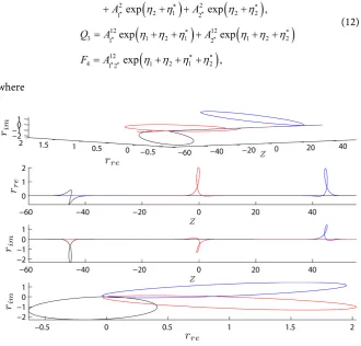
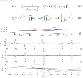
[image:6.595.209.539.391.660.2]

We then write the following expressions of F and Q with all coefficients, where exp

( )

η

∗j₀ =1. This leads to the three-rotating soliton solution depicted in

Figure 3.

Figure 3. From left to right panels rotating three-loop soliton solution to the CIDE Equation (1): For left we depict at times t= −30_{(blue color),}_t_{= 0 (red color) and}_t_{= 30}

(black color) corresponding to three moving states, with v1=2, v2=0.30, v3=0.55

and the computed angular velocities of such wave is Ω =1 0.25, Ω =2 1.00, Ω =3 0.50,

(7)

(

)

(

)

(

)

(

)

(

)

1 1 2

1 1 1 2 1 2

1 1 2

3 1 3 2

1 2 3

1 2 3 1 2 3

1 2 3 3 3 3 3

1 1 2

1 0 1 2 1

0 1

3 1 3 2

3 0 3 1

1 2 3 1 2 3 3 3 2

1 exp exp

exp , exp exp e C C C C C C C C C C C C

i i i

i j i i j j

j j j

i i i

i i i j j j

j j j

i i i

i j i i j

j j

i i i j j

F A A

A

Q A A

A

η η η η η η

η η η η η

∗ ∗ ∗ ∗ ∗ ∗ ∗ ∗ ∗ ∗ ∗ ∗ ∗ ∗ ∗ ∗ ∗ ∗ = + + + + + + + + + + + + = + + + + +

∑

xp

(

η ηi1 i2 ηi3 ηj1 ηj2

)

,

∗ ∗

+ + + +

(20)

(

)

1 1

0 1, 1 1,2,3 ,

i i

j

A∗=A = i =

(

)

1 1 1 1 1 2 1 1,2,3

1 _, _,

1,2,3 4 i j i j i A j

ω ω

∗ ∗ =   = _ _ =   +

(

)

1 2 1 2

1 2

1 1 1

2 ₁ ₂ ₁

1

1,2; 1

4 ,

1,2,3 i i i i

i i

j j j

i i i

A A A

j ω ω ∗ ∗ ∗ = = +   = − _ _ =  

(

) (

)

1 2 1 1 2 2

1 2 1 2

1 2 1 2 1 2

2 2 ₁ ₂ ₁

2

1 2 1

1,2; 1

4 , ,

1,2; 1

i i i i i i

i i j j

j j j j j j

i i i

A A A A A

j j j

ω ω ω ω

∗ ∗ ∗ ∗ ∗ ∗ ∗ ∗ = = +   = − − _ _ = = +  

(

)

(

)

(

) (

)

1 2 3 1 1 2 2 3 3

1 2 1 3

1 2 1 2 1 2 1 2

2 3 1 2

2 2

4

2 2 ₁ ₂ ₃

1 2 1

4

1; 2; 3

, ,

1,2; 1

i i i i i i i i i

i i i i

j j j j j j j j

i i j j

A A A A A A A

i i i

j j j

ω ω ω ω

∗ ∗ ∗ ∗ ∗ ∗ ∗ ∗ ∗ ∗ = − − = = =   × − − _ _ = = +  

(

)

(

) (

)

(

)

(

) (

)

1 2 3 1 1 1 2 2 2 3 3 3

1 2 1 3 2 3

1 2 3 1 2 3 1 2 3 1 2 3

1 2 1 3 2 3

2 2

2 6

2 2

2 ₁ ₂ ₃

1 2 3

4

1; 2; 3

, .

1; 2; 3

i i i i i i i i i i i i

i i i i i i

j j j j j j j j j j j j

j j j j j j

A A A A A A A A A A

i i i

j j j

ω ω ω ω ω ω

∗ ∗ ∗ ∗ ∗ ∗ ∗ ∗ ∗ ∗ ∗ ∗ ∗ ∗ ∗ ∗ ∗ ∗ = − − − = = =   × − − − _ _ = = =   (21)

• _Case_N_{= 4}

In this case the four-rotating soliton solution is obtain by

(

)

(

)

(

)

(

)

1 1 2

1 1 1 2 1 2

1 1 2

4 1 4 2

1 2 3

1 2 3 1 2 3

1 2 3 4 3 4 3

1 2 3 4

1 2 3 4 1 2 3 4

1 2 3 4 4 4 4 4

,

1 exp exp

exp exp , C C C C C C C C

i i i

i j i i j j

j j j

i i i

i i i j j j

j j j

i i i i

i i i i j j j j

j j j j

F A A

A

η η η η η η

η η η η η η η η

∗ ∗ ∗ ∗ ∗ ∗ ∗ ∗ ∗ ∗ ∗ ∗ ∗ ∗ ∗ ∗ ∗ ∗ ∗ ∗ = + + + + + + + + + + + + + + + + + + + +

∑

(

)

(

)

(

)

(

)

1 1 2

1 0 1 2 1

0 1

4 1 4 2

4 0 4 1

1 2 3

1 2 3 1 2

1 2 4 3 4 2

1 2 3 4

1 2 3 4 1 2 3

1 2 3 4 4 4 3 exp exp exp exp , C C C C C C C C

i i i

i j i i j

j j

i i i

i i i j j

j j

i i i i

i i i i j j j

j j j

Q A A

A

η η η η η

η η η η η η η

∗ ∗ ∗ ∗ ∗ ∗ ∗ ∗ ∗ ∗ ∗ ∗ ∗ ∗ = + + + + + + + + + + + + + + + +

∑

(22)

(

)

1 1

0 1, 1 1,2,3,4 ,

i i

j

A∗=A = i =

(

)

1 1 1 1 1 2 1 1,2,3,4

1 _, _,

(8)

(

)

1 2 1 2

1 2

1 1 1

2 ₁ ₂ ₁

,

1

1,2,3; 1

4 , ,

1,2,3,4

i i i i

i i

j j j

i i i

A A A

j ω ω ∗ ∗ ∗ = = +   = − _ _ =  

(

) (

)

1 2 1 1 2 2

1 2 1 2

1 2 1 2 1 2

2 2 ₁ ₂ ₁

, 2

,

1 2 1

1,2,3; 1

4 , ,

1,2,3; 1

i i i i i i

i i j j

j j j j j j

i i i

A A A A A

j j j

ω ω ω ω

∗ ∗ ∗ ∗ ∗ ∗ ∗ ∗ = = +   = − − _ _ = = +  

(

)

(

)

(

) (

)

1 2 3 1 1 2 2 3 3

1 2 1 3

1 2 1 2 1 2 1 2

2 3 1 2

2 2

, , 4

2 2 ₁ ₂ ₁ ₃ ₂

1 2 1

4

1,2; 1; 1

, ,

1,2,3; 1

i i i i i i i i i

i i i i

j j j j j j j j

i i j j

A A A A A A A

i i i i i

j j j

ω ω ω ω

∗ ∗ ∗ ∗ ∗ ∗ ∗ ∗ ∗ ∗ = − − = = + = +   × − − _ _ = = +  

(

)

(

) (

)

(

)

(

) (

)

1 2 3 1 1 1 2 2 2 3 3 3

1 2 1 3 2 3

1 2 3 1 2 3 1 2 3 1 2 3

1 2 1 3 2 3

2 2

2

, , 6

, ,

2 2

2 ₁ ₂ ₁ ₃ ₂

1 2 1 3 2

4

1,2; 1; 1

, ,

1,2; 1;

i i i i i i i i i i i i

i i i i i i

j j j j j j j j j j j j

j j j j j j

A A A A A A A A A A

i i i i i

j j j j j

ω ω ω ω ω ω

∗ ∗ ∗ ∗ ∗ ∗ ∗ ∗ ∗ ∗ ∗ ∗ ∗ ∗ ∗ ∗ ∗ ∗ = − − − = = + = +   × − − − _ _ = = + =  

(

)

(

)

(

)

(

) (

)

(

) (

)

(

) (

)

1 2 3 4 1 1 1 2 2 2 3 3 3 4 4 4

1 2 1 3

1 2 3 1 2 3 1 2 3 1 2 3 1 2 3

1 4 2 3 2 4 3 4 1 2

1 3 2 3

2 2

, , , 9 , ,

2 2

2 2 2

2 2 ₁ ₂ ₃ ₄

1

4

1; 2; 3; 4

,

i i i i i i i i i i i i i i i i

i i i i

j j j j j j j j j j j j j j j

i i i i i i i i j j

j j j j

A A A A A A A A A A A A A

i i i i

j

ω ω ω ω

ω ω ω ω ω ω ω ω ω ω

ω ω ω ω

∗ ∗ ∗ ∗ ∗ ∗ ∗ ∗ ∗ ∗ ∗ ∗ ∗ ∗ ∗ ∗ ∗ ∗ ∗ ∗ ∗ = − − × − − − − − = = = = × − −

2 1 3 2

,

1,2; j j 1; j j 1

 

 ₌ _{= +} ₌ ₊ 

 

(

)

(

) (

)

(

) (

)

(

) (

)

(

)

1 2 3 4 1 1 1 1 2 2 2 2 3 3 3 3 4 4 4 4 1 2 3 4 1 2 3 4 1 2 3 4 1 2 3 4 1 2 3 4

1 2 1 3 1 4 2 3 2 4

3 4 1 2 1 3 1

, , , 12 , , ,

2 2

2 2 2

4

i i i i i i i i i i i i i i i i i i i i

j j j j j j j j j j j j j j j j j j j j

i i i i i i i i i i

i i j j j j j

A A A A A A A A A A A A A A A A A

ω ω ω ω ω ω ω ω ω ω

ω ω ω ω ω ω ω

∗ ∗ ∗ ∗ ∗ ∗ ∗ ∗ ∗ ∗ ∗ ∗ ∗ ∗ ∗ ∗ ∗ ∗ ∗ ∗ ∗ ∗ ∗ ∗ = × − − − − − × − − −

(

)

(

)

(

)

(

)

4 2 3

2 4 3 4

2 2

2

2 ₁ ₂ ₃ ₄

1 2 3 4

1; 2; 3; 4

, .

1; 2; 3; 4

j j j

j j j j

i i i i

j j j j

ω ω ω

ω ω ω ω

[image:8.595.211.535.69.468.2]

∗ ∗ ∗ ∗ ∗ ∗ ∗ ∗ − − = = = =   × − − _ _ = = = =   (23)

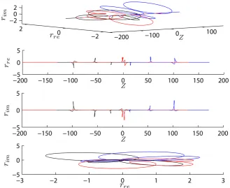
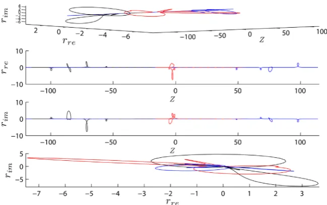
Figure 4 gives the depiction of the four-rotating soliton solutions to the CIDE.

4. Summary and Discussion

(9)

[image:9.595.211.536.68.272.2]

Figure 4. From left to right panels rotating four-loop soliton solution to the CIDE

Equa-tion (1): For right we depict at times t= −90_{(blue color),}t=0_{(red color) and}

90

t= _{(black color) corresponding to three moving states, with}v₁=0.91, v2=1.82,

3 1.33

v = _, v₄=1.11_{and the computed angular velocities of such wave is} Ω =₁ 0.015

and Ω =2 0.050, Ω =3 0.090, Ω =4 0.990 respectively.

Acknowledgements

The authors would like to express their sincere thanks to the anonymous referees for their critical comments and appropriate suggestions which have made this paper more precise and readable.

References

[1] Ablowitz, M.J. and Clarkson, P.A. (1991) Solitons, Nonlinear Evolution Equations

and Inverse Scattering. Cambridge University Press, New York. https://doi.org/10.1017/CBO9780511623998

[2] Malomet, B.A. (1992) Bound Solitons in Coupled Nonlinear Schrdinger Equations.

Physical Review A, 45, 8321-8323. https://doi.org/10.1103/PhysRevA.45.R8321

[3] Nakkeeran, D.J. and Porsesian, K.J. (1995) Solitons in an Erbium-Doped Nonlinear

Fibre Medium with Stimulated Inelastic Scattering. Journal of Physics A:

Mathe-matical and General, 28, 3817-3823. https://doi.org/10.1088/0305-4470/28/13/025

[4] Konopelchenko, B.G. and Magri, F. (2007) Coisotropic Deformations of Associative

Algebras and Dispersionless Integrable Hierarchies. Communications in

Mathe-matical Physics, 274, 627-658. https://doi.org/10.1007/s00220-007-0295-2

[5] Kakuhata, H. and Konno, K. (1997) Canonical Formulation of a Generalized

Coupled Dispersionless System. Journal of Physics A: Mathematical and General,

30L, 401-407. https://doi.org/10.1088/0305-4470/30/12/002

[6] Aoyama, S. and Kodama, Y. (1994) Topological Conformal Field Theory with a

Ra-tional Potential and the Dispersionless KP Hierarchy. Modern Physics Letters A, 9,

2481-2492. https://doi.org/10.1142/S0217732394002355

[7] Hassan, M.J. (2009) Darboux Transformation of the Generalized Coupled

Disper-sionless Integrable System. Journal of Physics A: Mathematical and Theoretical, 42,

(10)

[8] Konno, K. and Oono, H. (1994) New Coupled Integrable Dispersionless Equations. Journal of the Physical Society of Japan, 63, 377-378.

https://doi.org/10.1143/JPSJ.63.377

[9] Kakuhata, H. and Konno, K. (1996) A Generalization of Coupled Integrable,

Dis-persionless System. Journal of the Physical Society of Japan, 65, 340-341.

https://doi.org/10.1143/JPSJ.65.340

[10] Kotlyarov, V.P. (1994) On Equations Gauge Equation Uivalent to the Sine-Gordon

and Pohlmeyer-Lund-Regge Equations. Journal of the Physical Society of Japan, 63,

3535-3537. https://doi.org/10.1143/JPSJ.63.3535

[11] Novikov, S.P., Manakov, S.V., Pitaevskii, L.P. and Zakkarov, V.E. (1984) Theory of

Solitons, The Inverse Scattering Method. Consultant Bureau, New York.

[12] Konno, K. and Kakuhata, H. (1996) Novel Solitonic Evolutions in a Coupled

In-tegrable, Dispersionless System. Journal of the Physical Society of Japan, 65, 713-

721. https://doi.org/10.1143/JPSJ.65.713

[13] Levi, D. (1988) On a New Darboux Transformation for the Construction of Exact

Solutions of the Schrodinger Equation. Inverse Problem, 4, 165-172.

https://doi.org/10.1088/0266-5611/4/1/014

[14] Matveev, V.B. and Salle, M.A. (1991) Darboux Transformations and Solitons.

Springer, Berlin. https://doi.org/10.1007/978-3-662-00922-2

[15] Hirota, R. (2004) The Direct Method in Soliton Theory. Cambridge University

Press, Cambridge. https://doi.org/10.1017/CBO9780511543043

[16] Hirota, R. and Ohtam, Y. (1991) Hierarchies of Coupled Soliton Equations. I.

Jour-nal of the Physical Society of Japan, 60, 798-809. https://doi.org/10.1143/JPSJ.60.798

[17] Ma, W.X. and You, Y.C. (2005) Solving the Korteweg-de Vries Equation by Its

Bili-near Form: Wronskian Solutions. Transactions of the American Mathematical

So-ciety, 357, 1753-1778. https://doi.org/10.1090/S0002-9947-04-03726-2

[18] Ma, W.X. and Maruno, K.I. (2004) Complexiton Solutions of the Toda Lattice

Equ-ation. Physica A, 343, 219-237. https://doi.org/10.1016/j.physa.2004.06.072

[19] Geng, X.G. (2003) Algebraic-Geometrical Solutions of Some Multidimensional

Nonlinear Evolution Equations. Journal of Physics A—Mathematical and General,

36, 2289-2303. https://doi.org/10.1088/0305-4470/36/9/307

[20] Kakuhata, H. and Konno, K. (1999) Loop Soliton Solutions of String Interacting

with External Field. Journal of the Physical Society of Japan, 68, 757-762. https://doi.org/10.1143/JPSJ.68.757

[21] Kakuhata, H. and Konno, K. (2002) Rotating Loop Soliton of the Coupled

Disper-sionless Equations. Theoretical and Mathematical Physics, 133, 1675-1683.

https://doi.org/10.1023/A:1021366309313

[22] Kuetche, V.K., Bouetou, T.B. and Kofane, T.C. (2008) On Exact N-Loop Soliton

Solution to Nonlinear Coupled Dispersionless Evolution Equations. Physics Letters

A, 372, 665-669. https://doi.org/10.1016/j.physleta.2007.08.023

[23] Kuetche, V.K., Bouetou, T.B. and Kofane, T.C. (2007) Comment on Loop Soliton

Solutions of String Interacting with External Field? Journal of the Physical Society

(11)

Submit or recommend next manuscript to SCIRP and we will provide best service for you:

Accepting pre-submission inquiries through Email, Facebook, LinkedIn, Twitter, etc. A wide selection of journals (inclusive of 9 subjects, more than 200 journals)

Providing 24-hour high-quality service User-friendly online submission system Fair and swift peer-review system

Efficient typesetting and proofreading procedure

Display of the result of downloads and visits, as well as the number of cited articles Maximum dissemination of your research work