Journal of Mathematical Finance,2013, 3, 312-322
http://dx.doi.org/10.4236/jmf.2013.32031 Published Online May 2013 (http://www.scirp.org/journal/jmf)
Recent Developments in Fuzzy Sets Approach in
Option Pricing
Srimantoorao S. Appadoo1*, Aerambamoorthy Thavaneswaran2 1
Department of Supply Chain Management, University of Manitoba, Winnipeg, Canada 2
Department of Statistics, University of Manitoba, Winnipeg, Canada Email: *[email protected]
Received January 24, 2013; revised February 27, 2013; accepted March 21, 2013
Copyright © 2013 Srimantoorao S. Appadoo, Aerambamoorthy Thavaneswaran. This is an open access article distributed under the Creative Commons Attribution License, which permits unrestricted use, distribution, and reproduction in any medium, provided the original work is properly cited.
ABSTRACT
Recently there has been growing interest in fuzzy option pricing. Carlsson and Fuller [1] were the first to study the fuzzy real options and Thavaneswaran et al. [2] demonstrated the superiority of the fuzzy forecasts and then derived the membership function for the European call price by fuzzifying the interest rate, volatility and the initial value of the stock price. In this paper, we discuss recent developments in fuzzy option pricing based on Black-Scholes models. Fuzzy coefficient Black-Scholes partial differential equations (PDE) are derived. Membership function of the call price is given. The asset-or-nothing option by fuzzifying the maturity value of the stock price using adaptive fuzzy numbers is also discussed in some detail.
Keywords: Membership Function; Fuzzy Coefficient; Black-Scholes Partial Differential Equations (PDE); Asset-or-Nothing Option; Fuzzy Real Options
1. Introduction
Most stochastic models involve uncertainty arising mainly from lack of knowledge or from inherent vague-ness. Traditionally those stochastic models are solved using probability theory and fuzzy set theory. There exist many practical situations where both types of uncertain-ties are present. For example, if the price of an option depends upon the nature of the volatility which changes randomly, then the volatility of the stock price movement which is estimated from the sample data is a random variable as well as a fuzzy number. Recently there has been a growing interest in using fuzzy numbers to deal with impreciseness (see Appadoo et al. [3] and Thava-neswaran et al. [4] for more details). Many authors have tried to deal fuzziness along with randomness in option pricing models. For example, recently, Cherubini [5] determined the price of a corporate debt contract and provided a fuzzified version of the Black and Scholes model by means of a special class of fuzzy measures. On the other hand, Ghaziri et al. [6] introduced artificial in-telligence approach to price the options, using neural networks and fuzzy logic. They compare the result of artificial intelligence approach to that of Black-Scholes
model, using stock indexes. Since the Black-Scholes op-tion pricing formula is only approximate, which leads to considerable errors, Trenev [7] obtained a refine formula for pricing options. Due to the fluctuation of financial market from time to time, some of the input parameters in the Black-Scholes formula cannot always be expected in the precise sense. As a result, Thavaneswaran et al. [4] applied fuzzy approach to the Black-Scholes formula. Zmeskal [8] applied Black-Scholes methodology of ap-praising equity of a European call option by using the input data in a form of fuzzy numbers. Carlsson and Fuller [9] use possibility theory to study fuzzy real option valuation. Applications of fuzzy sets theory to volatility models have been studied by Thavaneswaran et al. [2] and Thiagarajah et al. [10]. Weidong et al. [11] discuss the analytical solutions for a European option using a fuzzy normal jump-diffusion model and possibility the-ory. Shiu and Shu [12] propose a fuzzy approach for in-vestment project valuation in uncertain environments from the aspect of real options. Guerra et al. [13] con-sider the Black and Scholes option pricing model, and present a sensitivity analysis based on the study of the option price when the parameters are supposed to be fuzzy numbers. Zdenek [8] proposed a generalized hy-brid fuzzy-stochastic binomial American real option
model under fuzzy numbers and Decomposition principle where the Input data are in a form of fuzzy numbers. Xu et al. [14] discuss three different versions of the Garman- Kohlhagen model, the put-call parity relationship and the calculation formulas of the Greek letters according to these three different G-K models based on fuzzy set the-ory. The empirical results indicate that the Greeks calcu-lated under fuzzy environment is a useful tool for man-aging option risk for an option writer. Nowak and Ro-maniuk [15] propose the method for option pricing based on application of stochastic analysis and theory of fuzzy numbers. The process of underlying asset trajectory be-longs to a subclass of Levy processes with jumps. Thiag-arajah et al. [10] present the Black-Scholes option pric-ing formula with quadratic adaptive fuzzy numbers, their approach hinges on a characterization of imprecision by means of fuzzy set theory.
1.1. Black-Scholes Model
The famous formula of Black-Scholes for the fair prices of European options follows from several assumptions, which are discussed in Metron [16]. Asset prices t are assumed to follow geometric Brownian motion and rep-resented by the equation
S
dSt S ttd S Wtd t, (1.1)
where the process Wt is a standard Brownian motion,
is the drift and is the volatility of the underlying stock. Generally, a call (put) option is the right to buy (sell) a particular asset for a specified amount at the strike price K at a specified time in the future with the expiration time T. If the option is of such a type that it can be exercised only on the expiration date itself, then it is called a European option. Let T be the price of the underlying asset at expiration time T. Then the payoff, g, of a European style call option at time T is given by
S
T max
T , 0
T
.g S S K S K (1.2)
This means that the call option is exercised if T and is abandoned otherwise. The above mentioned call and put options are sometimes called plain vanilla or standard options. Let be the risk-free interest rate. Then a probability measure Q is called an equivalent martingale measure to the probability measure for the discounted price process if
S K
P r
e rt
t t
S S
|
Q t s s
E S F S (1.3)
for each s t T
StQ
t
and , where is the history of the process up to time . This is the discounted price process which is a martingale under the probabil-ity measure . According to the Fundamental Theorem of Asset Pricing, an arbitrage-free price of an option at time is given by the conditional expectation of the
discounted payoff under an equivalent martingale meas-ure ,
~
Q P
t
t
F
t
C
Q
e r T t
t Q T t
C E g S F. (1.4)
Together with this equivalent martingale approach one needs a so-called equivalent portfolio (a combination of other traded assets). Then the price of the option has to coincide with the price of the corresponding equivalent portfolio. Following the results of Black-Scholes, we take a geometric Brownian motion as a stochastic proc-ess for modeling the stock price. This model is based on the assumption that the log-returns
1
log log
t t t
X S S (1.5)
are normally distributed. Now Equation (1.1) becomes
2 2 0e
t
W t
t
S S
(1.6)
0 t T. Using Itos lemma the model can equivalently be described as
dStS ttd S Wtd t. (1.7)
For this model, there exists a unique martingale meas-ure Q which is given by Girsanov’s theorem
2 2 dexp .
d T 2
r
Q r
W P
T (1.8)
Some calculations yield the Black-Scholes formula as,
2 0
0
2 0
log
2
log
2 e
BS
r S
r K
C S
S r K K
(1.9)
where denotes the cumulative distribution function of a standard normal variable, and T t denotes the time to expiration. In the literature two different ways of calculating volatility have been discussed. The first method is the empirical estimation from the historical data. The second is to calculate the implied volatility by equating the theoretical call price from the Black-Scholes formula with the market price.
loan. It is natural to take the rates on Treasury Bills and Treasury bonds, the government securities considered essentially default-free, as natural proxy for a risk-free discount rate for option payoffs. Yet, in practice, over- the-counter derivative traders consider LIBOR rates rather than the government rates as the appropriate cost of capital. LIBOR stands for London Interbank Offer Rate, an interest rate quote by a large bank at which it offers large short-term deposits to other banks. A corre-sponding bid rate, the rate at which banks accept deposits, is called LIBID. The difference between the sale (ask) and the buy (bid) prices for deposits is analogous to bid-ask spreads in the dealer markets for other securities, e.g., stocks. The existence of the bid-ask spread implies that the true market price is unknown. The bid-ask spread is considered a natural band to represent the uncertainty around the market price. In most empirical work, market prices, either for borrowing/lending or share purchases, are approximated by the mid-point of the bid-ask spread. This procedure among other things introduces errors into model-implied option prices. Another issue is the non- synchronous record of an option price and the price of the underlying asset. To top it off, true options them-selves are traded at bid/ask prices. Using models that do not specifically account for these issues introduces er-rors-difference between theoretical and observed option premiums. Thavaneswaran et al. [2] modelled the uncer-tainty of interest rate and stock price using fuzzy num-bers.
The rest of this paper is organized as follows. In Sec-tion 2, we study the Black-Scholes partial differential equations. Section 3 discusses the asset or nothing option. Section 4 closes the paper with conclusions.
1.2. Preliminaries and Notation
Before discussing the possibilistic moment generating function, we introduce some definitions and properties about fuzzy sets theory with relevant operations.
Definition 1.1 A fuzzy set A in , where is the set of real numbers, is a set of ordered pairs
xR R
, :
A x x xX , where
x is the membership function or grade of membership, or degree of compati-bility or degree of truth of xX which maps xXreal interval [0,1]. on the
Definition 1.2 A fuzzy set A in is said to be a convex fuzzy set if its
n
R
-level set A
are (crisp) convex sets for all
0,1 . Alternatively, a fuzzy setA in n is a convex fuzzy set if and only if for all and
R
n
R
1 2
x x, 0 1,
1 1 2
Min
1 ,
A x x A x A 2
x
Definition 1.3 A fuzzy number is called a trapezoidal fuzzy number (Tr.F.N.) with core
AF
a b, , leftwidth and right width if its membership function has the following form (see Figure1 for detail):
1 i
1 i
1 i
o f
f
f
0 therwise
a x
a x
a x b
g x
x b
a x b
(1.10)
and we use the notation A
a b, , , . It can easily be shown that
1 2
,
1 , 1
0,1 .
A a a
a b
(1.11)
The support of A is
a,b
. Moreover, for any fuzzy number A and a positive real number C, where the following relationship holds
1
1 2
0 d
AC
a a C. (1.12)Definition 1.4 Let be the set of all real numbers. A fuzzy number
R
, xG x R, is of the form
when ,
hen ,
en ,
therwise
1 w
wh
0 o
g x x a b
x b c G x
h x x c d
(1.13)
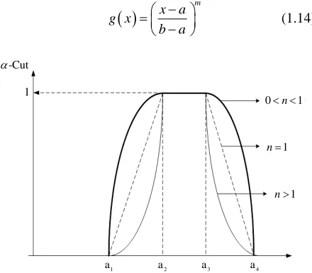
where g is a real valued, increasing and right continuous function, h is a real valued, decreasing and left continu-ous function, and a b c d, , , are real numbers such that
a b c d. A fuzzy number A with shape functions g and h defined by
x a m g xb a
(1.14)
1
a a2 a3 a4
-Cut
1
0 n 1
1
n
1
[image:3.595.316.536.523.716.2]n
d x n h xd c
(1.15)
respectively, where m or n0, will be denoted by
, , ,
m n,A a b c d . If m1 and n1, we simply write
, , ,
A a b c d m
, which is known as a trapezoidal fuzzy number. If 1 or n1, a fuzzy number
, * , , ,A a b c d m n is a modification of a trapezoidal fuzzy number A
a b c d, , ,
. If m1 and n1, then*
A is a concentration of A. Concentration of A by m 2
n is often interpreted as the linguistic hedge
“ve orn
1 hen *and
ry”. If 0
m , t A is a dilation of A. Dilation o A by n0.5 is often interpreted as the linguistic hedge “more or less”. Each fuzzy number A described by (1.14) and (1.15) has the follow gf m and
in - level sets (-level sets), A
a
,b
, a
,,
b R
0,1 and
1 0
, ,
, , , .
A g h
A b c A a d
1 1
If Aa b c d, , , m n, then, for all
0,1 ,
m1
, 1n
A a ba d dc
. (1.16)
1.3. Weighted Possibilistic Moments (WPM)
In this section following Carlsson and Fuller [1], we in-troduce the following moments. The first order f-WPM (or weighted possibilistic mean) of AF is given by
1
1 2
0d 2
f
a a
M A
f (1.17)where f
is a weight function such that
1 0d 1
f
.Similarly, the centered WPM (or weighted variance) of AF is
1
2 2
1 2
0 1
d 2
f
f f
Var A
f a M A a M A
(1.18) and for any positive integer r, the f-WPM of order r about the possibilistic mean value of A is defined as
1
1 2
0
1
d 2
r
r r
f f
E A
f a M A a M A
(1.19)
In analogy with Thavaneswaran et al. [4], the f- Weighted possibilistic skewness and the f-Weighted
pos-sibilistic kurtosis of a fuzzy number A are defined as
3Skewness
Var
f f
f
E A M A
A
A
and
4
2 2A E A
K
E A
. The f-Weighted possibilistic
co-variance between two fuzzy numbers A and B is given by
1
1 1
0
2 2
Cov ,
1 2
d
f
f f
f f
A B
f a M A b M B
a M A b M B
(1.20)
where f
is a weight function such that
1 10 d
f
.In analogy with Thavaneswaran et al. [4], the f-Weighted possibilistic skewness of fuzzy number A is defined as
3
32
Skewness A E A
E A
and similarly, the f-Weighted
possibilistic kurtosis of A is defined as Kurtosis
A
4
2 2E A
E A
f
. If x is an increasing function the -
level sets is given by f A
. Now,
1 2
1 , 2
f A f x x A
f x A x A
f A f A
(1.21)
On the other hand if f x
is a decreasing function the -level sets is given by f A
. Now,
2 1
2 , 1
f A f x x A
f x A x A
f A f A
(1.22)
Theorem 1.1Let A and B be two fuzzy numbers and
and positive numbers. Then, we have the
follow-1) ing results
,f f f
M AB M A M B
2) Varf
AB
2Var 2Var 2 Cov , ,
f A f B f A
B
3) Varf
AB
2 2
Varf A Varf B 2 Covf A,
,
4) Cov
,
Var
Var
4f f
f
A B A
A B B
.
A be a fuzzy number whose Let
option with terminal time T and payout is given by
Th S
, , t
f t S where f t x
, is the solution of the PDE-cuts are given by
1 , 2
a a for 0 1
, then the zero centered
bilistic t generating function is defined as A
weighted possi momen
MGF t if exists
2 1
, , , , , ,
2
, , , , , ,
, .
t xx
x
f t x t x f t x
r t x xf t x r t x f t x
f T x h x
,
1 et a e MGF f 2
1 0 1
d , 2
0 1
t a
A t
(1.23)2. Fuzzy Coefficient Black-Scholes PDE
and
d ,
where all of the model coefficients
, ,
f t x and its derivatives may be used to provide explicit formulas for the portfolio weights and t for the self-financing condition portfolio
t a
b b
t t t t a S that replicates h S
T .t t t t
V a S bt Consider the stock and bond model given by
From the self-financing condition and the models for the stock and bond, we have
dSt t S, t dt , ,t St dWt
d d d
, d , d , d
, , d ,
t t t t t
t t t t t t
t t t t t t t
V a S b
a t S t t S W b r t S
a t S b r t S t a t S dW.
t
t t
dt r t S, t t t
t S, t
,
, ,t St
,possibly and r t S
, t
are given by explicit function (fu ates) o the current time and current stock price. Then the arbitrage price at time t of a European
zzy estim From our assumption that Vt f t S
, t
and the Ito sˆformula f
2
2 1
, , , , , , , , , d , , , , d .
2
t t xx t t x t t x t t t
2 1
dVt ft , ,t St dt fxx , ,t St , ,t St dt fx , ,t St dSt
f t S f t S t S f t S t S t f t S t S W
The size of the stock portion of our replicating portfolio is:
, ,
.t x t
a f t S
2
, , , , , , , , , , , , .
2
t x t t t t t t xx t t x t t
t S f t S r t S b f t S f S t S f t S t S
The
terms cancel, and the bond portion is1 ,t
t S, t
fx , ,t St bt
,
, ,
2
, ,t t t
t t
b f t S f t
r t S
2
1 1
, , . xx St t St
Because Vt is equal to both f
, ,t St
and a St tbtt, the values for at and bt give us a PDE for f t S
, t
:
2
, ,
1 1
, , , , , , , , .
, 2
t t t t t t
x t t t t xx t t t
t t
V a S b
f t S S f t S f t S t S
r t S
f t S
Now, when we cancel
t
from the last term and re-place St by x, we arri he general Black-Scholes PD
ve at t da
E and its terminal boun ry condition. The portfolio weight at and bt for the self-financing portfolio
t t t t a S b
s
that replicates h S
T are explicitly givenabove. M over th same argument holds when we use fu mates for the unkn volatility parameter in
Suppose that the stock pays a dividend
ore e
zzy esti own
the model.
2.1. Fuzzy Coefficient Black-Sholes PDE with Dividends
,
t t
D k t S which is a function of the stock price St.
. t t t t t V a S b and
respectively, with the terminal boundary cond
,
ition
f T x h x for all xR.
Using cm argument, we arrive at the Black-Scholes PDE:
1 2 2
, , , ,
2
, , , , ,
t xx
x t
with its terminal boundary condition
f t x x f t x
rxf t x D
t x rf
,
f T x h x for all
2.2. Membership Functions of Call Price
rm
.
t
xR.
For the Black Scholes model of the fo
dStStdtS Wtd
For this model, there exists a unique martingale meas-ure Q which is given by Girsanov’s theorem
2dQ r r
2
exp .
dP WT 2 T
urrent stock price S
Solving the Black-Scholes PDE, the arbitrage price of the European call option at time t with c
2
2
log
2
log
2 e
BS
C S
r
S r K
S r K
K
where denotes the cumulative distribution unction of a st d normal variable, is the strike price, is th ry date and
andar e expi
f
K T
T t
that we ho is th ld
e residual time. Th
amount stock in the replicating p
folio at ti e
e of
m
t
a
is
t
2
log
2
t
t t t
S r K
a b
2
log
2
e .
t
r
S r K
K
We replace the fuzzy interest rate, the fuzzy stock price, and the fuzzy volatility by possibilistic mean value in the fuzzy Black-Scholes formula. The initial stock price cannot be characterized by a single number. Thus, we assume that the initial stock price is a fuzzy number of the form
0 1, 2, 3, 4
S S S S S . A fuzzy num f the
form
ber o
3
4 2 1
3
4 4 1 1
e e , e , e , e
e e e , e e e
r
r r r
r
r
r r r r
2
r
for the discounting factor in a fuzzy sense and of the form
1, 1, 3, 4
for the volatility can also be modeled in a similar manner. In these circumstances we suggest the use of the following fuzzy weighted possi-bilistic (heur ula as in Carlsson and Fuller [
istic) option 9] for computing fu the following Blac ng stock with exercise
form
zzy option values. We con-sider k-Scholes formula for a dividend
payi price K.
0e 1 e 2
r ,
FCOV S N d K N d (2.1)
where
2 0
1
ln
2
f f
f
f
M S M
M r
K d
M
, (2.2)
2 1 f
d d M , (2.3)
f
M x is the possibilistic mean value of variable x. ntinuously at We assume that the stock pays dividends co
n rate . The
a know -level sets of the fuzzy tion value
call op-
FCOV are as follows:
1 , 2 ,
FCOV FCOV FCOV (2.4)
where
1 e
e
FCOV
1
1 2
1 1 2
2 2 1 1
e
e e
r
r r
N d S KN d
KN d S S N d
(2 )
.5
4
3 4
2
1 4 2
4 3 1 2
e e
e e
r
r r
FCOV
N d S KN d
S S N d KN d
e
(2.6)
1
1 2
1 2
3 2
4
3 4
1 1 2
1 2 2 1 2
2 2 1 1
2 1 2 3 1 2
1 4 2
4 3 1 2
e e
e , e e
e e e
1 e e , e e
e e
e e e
r
r r
r r
r r
C
r
r r
C N d S KN d
d KN d S N d KN d
KN d S S N d
C S N d KN d S N d KN d
N d S KN d C
S S N d KN d
1
Se N
C
3 4
3e 1 2 e , 4e 1 2 e
0 otherwise
r r
C S N d KN d S N d KN d
In the following example we consider the fuzzy call price on a stock option using a fuzzy number discussed earlier.
Example 1 Consider a European call option on a stock with the following assumptions. The current stock
price, the stock price volatility and the risk-free interest rate are all taken Tr.F.N fuzzy numbers and
1 0
d 1, 1 n
f f n
.
158,160, 2, 2 , 0.03, 0.04, 0.01, 0.01 , 0.28, 0.29, 0.02, 0.03 , 2, 0.03, 140,
156 2 ,162 2 , 0.26 0.02 , 0.32 0.03 , 0.02 0.01 , 0.05 0.01
S r K
S r
57
115
200 2f
n M
n
1
156 2 162 21 d 159
2 n
f
M S n
0
1
0
0.02 0.01 0.05 0.01
1 d
2 n
f
M r n 7 0.035
200
2
1
159 1 57 115
ln 0.035 0.03 2
140 2 200 2
57 20
115 2 0 2
n n d
n n
2
2
57 115
159 1
ln 0.035 0.03 2
140 2 200 2 57 115
2 200 2
57 115
2 200 2
n
n n
d
n n
n
With the help of the above fuzzy expressions we price the ll in a fuzzy possibilistic setup. ca
0.03 2
0.02 2
0.02 2 0.03 2
0.03 2
1 e 1 156 140 2 e 140 2 e e 158 156 e
FCOV N d N d N d N d1
0.03 2
0.05 2
0.03 2
0.04 2 0.05 2
2 e 1 162 140 2 e 162 160 e 1 140 2 e e
FCOV N d N d N d N d
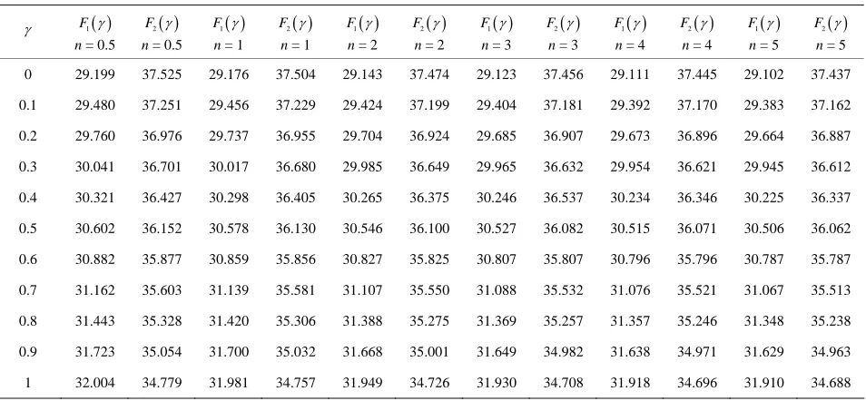
We present the fuzzy call option values for various levels of and n as in Table 1 and Figure 2. A fuzzy weighted possibilistic model is sufficiently flexible and can be easily adjusted or tuned for optimal solution. The flexibility is in the ability to choose different values of n
according to different criteria. For example, a bank could calibrate n to improv volatility forecasts, which are es-sential for Value-at-Risk calculations for option portfo-lios. Alternatively, the value of n can be trained to im-prove the precision of computed hedge ratios (Greeks).
Table 1. The fuzzy call option values for various levels of γ and n.
F1
n = 0.5
2
F n = 0.5
1
F n = 1
2
F n = 1
1
F n = 2
2
F n = 2
1
F n = 3
2
F n = 3
1
F n = 4
2
F n = 4
1
F n = 5
2
F n = 5 0 29.199 37.525 29.176 37.504 29.143 37.474 29.123 37.456 29.111 37.445 29.102 37.437 0.1 29.480 37.251 29.456 37.229 29.424 37.199 29.404 37.181 29.392 37.170 29.383 37.162
.924 .649 .375
.100 30.527 36.082 30.515 36.071 30.506 36.062
0.6 30.882 35.877 35.796 30.787 35.787
0. 31.162 35.603 31.139 35.581 31.107 35.550 31.088 35.532 31.076 35.521 31.067 35.513 0.8
0.
0.2 29.760 36.976 29.737 36.955 29.704 36 29.685 36.907 29.673 36.896 29.664 36.887 0.3 30.041 36.701 30.017 36.680 29.985 36 29.965 36.632 29.954 36.621 29.945 36.612 0.4 30.321 36.427 30.298 36.405 30.265 36 30.246 36.537 30.234 36.346 30.225 36.337 0.5 30.602 36.152 30.578 36.130 30.546 36
30.859 35.856 30.827 35.825 30.807 35.807 30.796 7
31.443 35.328 31.420 35.306 31.388 35.275 31.369 35.257 31.357 35.246 31.348 35.238 9 31.723 35.054 31.700 35.032 31.668 35.001 31.649 34.982 31.638 34.971 31.629 34.963 1 32.004 34.779 31.981 34.757 31.949 34.726 31.930 34.708 31.918 34.696 31.910 34.688
1
29.199 32 34.77 37.525
[image:8.595.58.295.107.525.2]Option Values
Figure 2. Membership function for different values on n and for 0 ≤ γ ≤ 1.
This may be beneficial for hedging performance, which is essential in risk management.
3. General Terminal-Value Claims
A standard option is a contract that gives the holder the right to buy or sell an underlying asset at a specified price on a specified date. The payoff depends on the un-derlying asset price. The call option gives the holder the right to buy an underlying asset at a strike price; th
er the underlying asset price, the more
tic call option with
dis-on s p . T tio d
m o th erlyin
he st pric ts e ion h w
b p ass ot ll a
-n c on. he pe pt s
off nothing if the underlying asset price ends up below
he pri r t nd th n ff
th rly se en be e
rike s a d am f i u
e pr te or a on
-sse e st d e as e
is termed the stock price. The method of pricing the European call option can be used to find the price of any
e strike price is termed a specified price or exercise price. Therefore the high
valuable the call option. If the underlying asset price falls below the strike price, the holder would not exercise the option. Binary option is an exo
c tinuou ayoffs he op n pays off a fixe , prede-ter
t
ined am rike
unt if e on i
e und xpirat
g asset pr date. T
ice is b ere are t
eyond o types of inary o tions: et-or-n hing ca option nd cash-or othing all opti For t first ty , the o ion pay
t strike ce. Fo he seco type, e optio pays o nothing if e unde ing as t price ds up low th st
th
price a strike
nd pay ice. No
fixe that f
ount i the bin
t ends ry opti
p above the un derlying a t is th ock an the und rlying set pric
claim in the Black-Scholes model:
dStS ttd S Wtd t,
that is
22
0e t
W t
t
S S ,
where and represent the expected return and volatility per unit time, respectively, and
Wt is aWiener process. The price at time 0 of a claim paying C at time T is eQ rTC
, where taking expectations with the martingale probability Q gives the same value as taking expectations with the original probabilities with the assumption that r; the price at time t will be
e r T t
Q C t
F
. Here C may be any FT random
variable with 2 C
. The following theorem gives the time t price of a general terminal-value claim
TC f S .
Theorem 3.1
v TC S for some real number v is
1
22
e v r v T t v
t
S ,
2) The time t price of the asset-or-nothing claim
v
T T
C S I a S b is
1 1 2
2v r v v T t
v v
S d b d a
, (3.1)
1
e
v
where t
2 u
t ln
2 t
v
r T t
S
d u v T
T t
,
and a
and b
are the upper and lower - cuts, respectively.3) For any twice differentiable function
: 0,
f R, the time t price of the terminal value claim C f
ST
I a
ST b
is g n by r T t
ive
, e
eX
T
p x t f x I a S b where
2
2
X Z T t r Tt ,
option stated the fuzzy concept is taken i to account in a model.
set as trapezoidal y mber with core
n fuzz
Proof: see A. Thavaneswaran et al. [18].
le 2 For the asset-or-nothing
Examp
above,
Define a fuzzy
S Sa, b
, left width and right width nu . Consider the toid function. By intro g the fuzzy concept ry function an investor m y have more oppor-tunities to think about his decision in some aspe me
the trapez into a bina
as risk.
mbership func ion related to asset price which follows ducin
a
ct such
1 if
1 if
1 if
0
b b
otherwise a
a a
a b
b
S S T
S S T S
S S T S
S T S
S S T S
g S T
(3.2)
0, 0
The mo at the ma
rlying asset p .
st possible values of th de rice turity date lie in the interval
e un
S Sa, b
, and Sb is the upward potential and Sa rly
is th ing as
e downwar r the values of the u set price.
d For potentia
fixin
l fo nde
g parameter values of , , Sa, and many ways to be considered. For example, whe
b S there
are n the
investor cannot predict how the underlying asset price changes at the maturity date, in other words, when he becomes confident that the asset price has fluctuated
he will take the range of sufficiently large width so that the premium values become high. On the other hand, when much fluctuation is not observed the width will become small, so that Sa gets equal to Sb, result-ing in triangular fuzzy numbers. For each of three sets the corresp
greatly
onding payoff tained by mu lying its grade of membership functio
is ob n,
ltip
s .
In this case, and the rlying asset moves between
unde S T
a
S and Sb . T as a
h dif
en, the value of
option m ference een the
presen
present ay be com
t value of
puted betw
whS T ich exceeds Sa and t of
hat
S T which is above Sb .
2
if
if
0 otherwise
a b
b
b b
S T S S T S
S T S S T
S T S S T S
2 payoff
a
a a
g S T S T
S S T S T
S T S
if S T S
Then, the values of asset-or-nothing option with fuzzy nature are as follows
1 2 3 CC C C
where
1 e ,
r T t Q
a b
C S T
S S T S
2
a Q Q
T t
a a
S S T S
C
S T S
2
e ,
T
r
S
2 T
nditio ion wi
r T
T
3 e ,
a Q b Q
r T t
b a
S S S T
C
S S T S
with appropriate boundary co ns, wh de-notes the conditional expectat th re o risk- neutral probability.
S
ere spect t
S
Q
1 e e
r T t t
Q Q
a b
C S T
S S T S
er T t St d Sb d Sa ,
2 2 2 2 2 1 2 1 2 2 12 2 2 2 | | e | | e e e e Q t
a Q t
r T t
Q t
a Q t
r T t r T t a
r T t
a t a a t a a
r T t
S T
S S T
C
S T
S S T S S T S T
S S d S d S S d S d S
F F F F
2 2 2 2 e e ,r T t
a t a a t a a
r T t
a a
S S d S d S S d S d S
S S T S
and
2 2 3 2 2 2 | | e e e .Q t b Q t
r T t
r T t
t b b b t b
r T t
S T S S T
C
S d S d S S S d S d S
F F b
Example 3 When we model the terminal value by an adaptive fuzzy number having membership function of the form: T S
1 if 1 if 1 if 0 otherwise n a a a a b n b b bS S T
S S T
S S T S
g S T
S T S
S S T S
S (3.3) and if the payoff is given by
if if 0 otherwise, n a b n b b bg S T S T
S S T S
S T S
S T S T S S T S
if
a
a a
S S T
S T S T S S T S
S T (3.4)
then the time t call price is given by 3 where 1 2
CC C C ,
1 e |
,
r T t
Q t
t b a
a b
C S T
S d S d S
S S T S
F and
2 0 e ( ) 1 e 1 e 1 e 1 nr T t a
Q t
n n
r T t a
Q t
n
n r T t
Q a t
n
n
k
r T t n k k
Q a
k
S T S
C S T
S S T
S T
S T S S T
n
S T S S T
k