An Application of Generalized Entropy Optimization Methods in Survival Data Analysis

(1)

ISSN Online: 2153-120X ISSN Print: 2153-1196

An Application of Generalized Entropy

Optimization Methods in Survival Data Analysis

Aladdin Shamilov

1

, Cigdem Kalathilparmbil

1*

, Sevda Ozdemir

2

1_{Faculty of Science, Department of Statistics, Anadolu University, Eskişehir, Turkey}

2_{Ozalp Vocational School, Accountancy and Tax Department, Yuzuncu Yil University, Van, Turkey}

Abstract

In this paper, survival data analysis is realized by applying Generalized En-tropy Optimization Methods (GEOM). It is known that all statistical distribu-tions can be obtained as MaxEnt distribution by choosing corresponding moment functions. However, Generalized Entropy Optimization Distribu-tions (GEOD) in the form of

MinMaxEnt,MaxMaxEnt

distributions which are obtained on basis of Shannon measure and supplementary optimization with respect to characterizing moment functions, more exactly represent the given statistical data. For this reason, survival data analysis by GEOD acquires a new significance. In this research, the data of the life table for engine failure data (1980) is examined. The performances of GEOD are established by Chi-Square criteria, Root Mean Square Error (RMSE) criteria and Shannon entropy measure, Kullback-Leibler measure. Comparison of GEOD with each other in the different senses shows that along of these distributions

(

MinMaxEnt

)

₄ is better in the senses of Shannon measure and of Kullback- Leibler measure. It is showed that,

(

MinMaxEnt

) (

3

(

MaxMaxEnt

)

4

)

is more

suitable for statistical data among

(

MinMaxEnt ,

)

_m m=1,2,3,4 MaxMaxEnt ,

(

)

_m m=1,2,3,4

)

. Moreover,

(

MinMaxEnt

)

₃ is better for statistical data than

(

MaxMaxEnt

)

₄ in the sense of RMSE criteria. According to obtained distribution

(

MinMaxEnt

)

₃

(

)

(

MaxMaxEnt 4

)

estimator of Probability Density Function f tˆ

( )

,

Cumula-tive Distribution Function F tˆ

( )

, Survival Function S tˆ

( )

and Hazard Rate

( )

ˆ

h t are evaluated and graphically illustrated. The results are acquired by us-ing statistical software MATLAB.

Keywords

Survival Function, Censored Observation, Generalized Entropy Optimization Methods,

MaxEnt,MinMaxEnt,MaxMaxEnt

Distributions

How to cite this paper: Shamilov, A., Kalathilparmbil, C. and Ozdemir, S. (2017) An Application of Generalized Entropy Optimization Methods in Survival Data Analysis. Journal of Modern Physics, 8, 349-364.

https://doi.org/10.4236/jmp.2017.83024 Received: August 5, 2016

Accepted: February 25, 2017 Published: February 28, 2017

http://creativecommons.org/licenses/by/4.0/

(2)

1. Introduction

Entropy Optimization Methods (EOM) have important applications, especially in statistics, economy, engineering and so on. There are several examples in the litera-ture that known statistical distributions do not conform to statistical data; however, the entropy optimization distributions conform well. Generalized Entropy Optimi-zation Methods (GEOM) have suggested distributions in the form of MinMaxEnt which is the closest to statistical data, and MaxMaxEnt which is the furthest from mentioned data in the sense of information theory [1][2], respectively. For this reason, GEOM can be more successfully applied in Survival Data Analysis.

Different aspects and methods of investigations of survival data analysis are considered in [3]-[8].

In particular in the paper [6], it is investigated several problems of hazard rate function estimation based on the maximum entropy principle. The potential ap-plications include developing several classes of the maximum entropy distribu-tions which can be used to model different data-generating distribudistribu-tions that sa-tisfy certain information constraints on the hazard rate function.

In order to represent the results of our investigations, we give some auxiliary concepts and facts first.

2. Survival Analysis

Survival time can be defined broadly as the time to the occurrence of a given

event. This event can be the development of a disease, response to a treatment, relapse or death [9].

Censoring: The techniques for reducing experimental time are known as

cen-soring. In survival analysis, the observations are lifetimes, which can be indefi-nitely long. So quite often the experiment is so designed that the time required for collecting the data is reduced to manageable levels.

Let T be a continuous, non-negative valued random variable representing the lifetime of a unit. This is the time for which an individual (or unit) carries out its appointed task satisfactorily and then passes into “failed’’ or “dead’’ state thereafter [10].

The probabilistic properties of the random variable are studied through its cumulative distribution function F or other equivalent functions defined be-low [9]:

Cumulative Distribution Function:

( )

{

}

₀t

( )

d , 0

F t =P T t< =

_∫

f u u < < ∞t

Survival Function: This function is denoted by

S t

( )

, is defined as the

proba-bility that an individual survives longer than t:

( )

1 ( )

S t

= −

F t

( )

{

}

_t

( )

d , 0

S t =P T t> =

_∫

∞f u u < < ∞t

Probability Density Function: Like any other continuous random variable, the

(3)

probability that an individual fails in the short interval t+ ∆t per unit width

t

∆ _{, or simply the probability of failure in a small interval per unit time. It can be} expressed as

( )

d

( )

d

( )

d d

F t S t f t

t t

= = −

Hazard Rate: This function is defined as the probability of failure during a

very small time interval, assuming that the individual has survived to the begin-ning of the interval, or as the limit of the probability that an individual fails in a very short interval, t+ ∆t, given that the individual has survived to time t:

( )

f t

_{( )}

( )

.

h t S t =

3. Generalized Entropy Optimization Methods (GEOM)

Entropy Optimization Problem (EOP) [11] and Generalized Entropy Optimiza-tion problem (GEOP) [10] can be formulated in the following form.

EOP: Let _f( )0

( )

_x _{be given probability density function (p.d.f.) of random}

variable X, L be an entropy optimization measure and g be a given mo-ment vector function generating m moment constraints. It is required to ob-tain the distribution corresponding to g, which gives extreme value to L.

GEOP: Let _f( )0

( )

_x _{be given probability density function of random variable}

X, L be an entropy optimization measure and K be a set of given moment vector functions. It is required to choose moment vector functions _g( )1 _,

( )2

g ∈K such that _g( )1 _{defines entropy optimization distribution}_f( )1

_{( )}

_x

closest to _f( )0

( )

_x _, _g( )2 _{defines entropy optimization distribution} _f( )2

( )

_x

furthest from _f( )0

( )

_x _{with respect to entropy optimization measure} _L_{. If} _L_is

taken as Shannon entropy measure, then _f( )1

( )

_x _{is called the} _MinMaxEnt_distri-

bution, and _f( )2

( )

_x _{is called the}_MaxMaxEnt_distribution_[1]_[2]_[12]_[13]_[14]_.

The method of solving GEOP is called as GEOM.

3.1. MaxEnt

Functional

The problem of maximizing entropy function

( )

1 ln ,

(

1, ,

)

n

i i n

i

H p = −

∑

₌ p p p= p  p (1)

subject to constraints

( )

1 1 1 , 0,1, 2, ,

n n

i i j i j

i= p = i= p g x =µ j= m

∑

 (2)

where

µ =

0

1,

g x

0

( )

=

1, 0, 1,2, , ; 1

p

i

≥

i

=



n m

+ <

n

,

has solution

( )

0 _{, 1, 2, ,}

m j j i j g x

i

p ₌e−∑ =λ i₌ _ n₍₃₎

where

λ

j

(

j

=

0,1,2, ,



m

)

are Lagrange multipliers. Finding the distribution

(

p p

1

,

2



,

p

n

)

which maximizes function (1) subject to constraints generated

(4)

the MATLAB program to calculate Lagrange multipliers.

If (3) is substituted into (1), the maximum entropy value is obtained:

( )

0 ( )

(

_{( )}

)

max 0

1 0

.

m j j i j

n _{g x} m

m

j j i j j j

i j

H p e− =λ λ g x λ µ

=

= =

∑

= −

_∑

−

∑

=

_∑

₍₄₎

If distribution ( )0

(

( )0 ( )0

)

1 , , n

p = p  p is calculated from the data, the moment

vector value

µ

=

(

1, ,

µ

1



µ

m

)

can be obtained for each moment vector function

( )

(

1, 1

( )

, , m

( )

)

g x = g x  g x . Thus, Hmax is considered as a functional of

g x

( )

and called the MaxEnt functional. Therefore, we use the notation

U g

( )

to denote the maximum value of H corresponding to

( )

(

1, 1

( )

, , m

( )

)

g x = g x  g x .

3.2. MinMaxEnt

and

MaxMaxEnt

Distributions

Let K be the compact set of moment vector functions

g x U g

( ) ( )

.

reaches its least and greatest values in this compact set, because of its continuity proper-ty. For this reason,

( )

( )1

_{( )}

( )

( )2

min ; max .

g K∈ U g =U g g K∈ U g =U g Consequently,

( )

1

( )

( )2 _.

U g ≤U g

Distributions ( )1

(

( )1 ( )1

)

1 , , n

p = p  p and ( )2

(

( )2 ( )2

)

1 , , n

p = p  p corresponding

to the _g( )1

( )

_x _and _g( )2

_{( )}

_x _{, respectively, are called} _MinMaxEnt_and

MaxMaxEnt distributions [1].

(

)

MinMaxEnt MaxMaxEnt

method for a finite set of characterizing moment functions can be defined in following form.

Let

K

0

=

{

g

1

, ,



g

r

}

be the set of characterizing moment vector functions

and all combinations of r elements of K0 taken m elements at a time be 0,m

K . We note that, each element of K0,m is vector g with m components.

Solving the MinMaxEnt and the MaxMaxEnt problems require to find vector functions

(

( )1

_{( )}

)

0,

g g x ,

(

( )2

_{( )}

)

0,

g g x , where

( )

( )1 ( )2

0 1, , 0,m 0,m

g x = g ∈K g ∈K minimizing and maximizing

U g

( )

accor-dingly with respect to Shannon entropy measure. It should be noted that

U g

( )

reaches its minimum value subject to constraints generated by function

g x

0

( )

and all m-dimensional vector functions

g x g K

( )

,

∈

0,m. In other words,

min-imum value of

U g

( )

is least value of values Hmax corresponding to

( )

,

0,m

g x g K

∈

_{. If}

(

( )1

)

0,

g g gives the minimum value to

U g

( )

then distribu-tion ( )1

(

( )1 ( )1

)

1 , , n

p = p  p corresponding to

(

( )1

)

0,

g g is called the

MinMaxEnt distribution. MinMaxEnt method represents probability distri-bution in the form of MinMaxEnt distribution. In a similar way,

U g

( )

reaches its maximum value subject to constraints generated by function

g x

0

( )

and all m-dimensional vector functions

g x g K

( )

,

∈

0,m. In other words,

max-imum value of

U g

( )

is greatest value of values Hmax corresponding to

( )

,

0,m

g x g K

∈

_{. If}

(

( )2

)

0,

g g gives the maximum value to

U g

( )

then distribu-tion ( )2

(

( )2 ( )2

)

1 , , n

p = p  p corresponding to

(

( )2

)

0,

(5)

MaxMaxEnt distribution. MaxMaxEnt method represents probability dis-tribution in the form of MaxMaxEnt distribution. It should be noted that both distributions can be applied in solving proper problems in survival data analysis.

4. Application of

MinMaxEnt

and

MaxMaxEnt

Methods

to Survival Data

4.1. MinMaxEnt

and

MaxMaxEnt

Distributions for Finite Set of

Characterizing Moment Functions

In the present research, the data of the life table for engine failure data (1980) given in Table 1 is considered [10].

In our investigation, the experiment is planned for 200 numbers of patients surviving at beginning of interval but the presence of censoring from the plan-ning patients 97 individuals stay out the experiment. This situation is taken into account in Table 2.

[image:5.595.206.538.345.528.2]

It should be noted that, the presence of censoring in the survival times leads to a situation where the sum of observation probabilities stands less than 1 for the

Table 1. The data of the life table for engine failure data (1980).

Survival Time (year) t

Working at the beginning of interval ni

Failed during the interval di

Censored during the interval ci

0 - 1 200 5 0

1 - 2 195 10 1

2 - 3 184 12 5

3 - 4 167 8 2

4 - 5 157 10 0

5 - 6 147 15 6

6 - 7 126 9 3

7 - 8 114 8 1

8 - 9 105 4 0

9 - 10 101 3 1

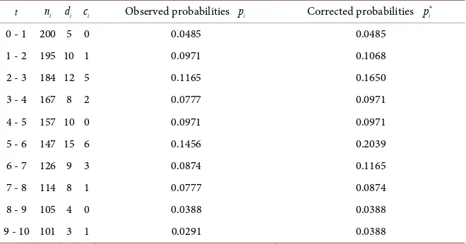
Table 2. Observed and corrected probabilities.

t ni di ci Observed probabilities pi Corrected probabilities pi ∗

[image:5.595.209.539.562.735.2]

(6)

survival data. For this reason, in solving many problems, it is required to sup-plement the sum of observation probabilities up to 1. Since the sum of observed probabilities pi in Table 2 is 0.8155, according to the number of censoring,

supplementary probability 1 0.8155 0.1845− = _{is uniformly distributed to each} censoring data and corrected probabilities

p

i∗ are obtained.

As we noted that above, MinMaxEnt and MaxMaxEnt distributions can be applied in solving proper problems in survival data analysis. In our investiga-tion as components of K0 characterizing moment vector function

( )

2

( )

( ) ( )

2

1 , , ln , ln2 3 4

g x =x g x =x g x = x g x = x ,

( )

(

2

)

5 ln 1

g x = +x are chosen. The set of moment functions is chosen from the characteristic moments which are mostly used in Statistics.

Consequently,

K

0

=

{

g

1

, ,



g

5

}

. For example, if m=3 then

( )

(

1

)

(

2

(

)

2

)

( )1 0, 1, , , ln , 0,3

g g = x x x g ∈K

gives the least value to

U g

( )

and

( )

(

2

)

(

2

(

2

)

( )2

0, 1, , ln , ln 1 , 0,3

g g = x x +x g ∈K

gives the greatest value to

U g

( )

.

The MaxEnt distributions corresponding to

(

g g g x

0

, ,

)

0

( )

=

1,

g K

∈

0,m

, 1,2, ,4

m

=



and Hmax values are shown in

Tables 3-6. In these tables, MinMaxEnt and MaxMaxEnt distributions cor-responding to HMinMax and HMaxMax are represented with bold font. By virtue

of these tables are also obtained

(

MinMaxEnt

)

_m,

(

MaxMaxEnt

)

_m,

1,2,3,4

m= distributions which are shown in Table 7 and Table 8.

In order to obtain the performance of the mentioned distributions, we use various criteria as Root Mean Square Error (RMSE), Chi-Square, entropy values of distributions. The acquired results are demonstrated inTable 9 and Table 10.

All

(

MinMaxEnt , MaxMaxEnt ,

) (

_m

)

_m

m

=

1,2,3,4

distributions are accepta-ble to survival data in the sense of Chi – Square criteria.

[image:6.595.206.541.585.735.2]

In the sense of RMSE criteria each

(

MinMaxEnt

) (

_m

m

=

1,2,3,4

)

_distribution is better than corresponding

(

MaxMaxEnt

) (

_m

m

=

1,2,3,4

)

_{distribution.} More-over,

(

MinMaxEnt

)

₁ is nearer to statistical data than

(

MaxMaxEnt

)

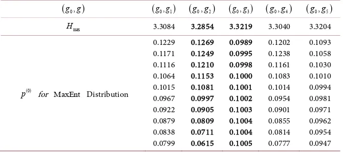
₁ and

Table 3. The predicted probabilities for the MaxEnt distribution corresponding to

(

g g g x0, ,

) ( )

0 =1,g K∈ 0,1 and Hmax values.

(

g g0,

)

(

g g0, 1

)

(

g g0, 2

)

(

g g0, 3

)

(

g g0, 4

)

(

g g0, 5

)

max

H 3.3084 3.2854 3.3219 3.3040 3.3204

( )0

p for MaxEnt Distribution

(7)

[image:7.595.210.538.107.398.2]

(

g g g x0, ,

) ( )

(

g g0,

)

(

g g g0, ,1 2

)

(

g g g0, ,1 3

)

(

g g g0, ,1 4

)

(

g g g0, ,1 5

)

(

g g g0, ,2 3

)

max

H 3.2042 3.2140 3.2921 3.2106 3.2041

( )0

0.0619 0.0921 0.1218 0.1434 0.1502 0.1400 0.1160 0.0856 0.0562 0.0328 0.0429 0.1137 0.1451 0.1490 0.1377 0.1194 0.0994 0.0803 0.0634 0.0492 0.0863 0.1449 0.1299 0.1126 0.0999 0.0914 0.0861 0.0833 0.0824 0.0832 0.0543 0.0939 0.1351 0.1529 0.1480 0.1290 0.1046 0.0804 0.0593 0.0424 0.0483 0.1036 0.1363 0.1493 0.1456 0.1296 0.1068 0.0820 0.0589 0.0397

(

g g0,

)

(

g g g0, ,2 4

)

(

g g g0, ,2 5

)

(

g g g0, ,3 4

)

(

g g g0, ,3 5

)

(

g g g0, ,4 5

)

max

H 3.2408 3.2057 3.2305 3.2500 3.2237

( )0

[image:7.595.207.540.444.737.2]

0.1101 0.0825 0.1058 0.1285 0.1396 0.1344 0.1150 0.0877 0.0598 0.0366 0.0579 0.0928 0.1281 0.1484 0.1499 0.1353 0.1108 0.0830 0.0573 0.0365 0.0400 0.1294 0.1481 0.1403 0.1251 0.1091 0.0944 0.0816 0.0706 0.0613 0.0423 0.1425 0.1432 0.1278 0.1134 0.1018 0.0924 0.0848 0.0785 0.0733 0.0403 0.1205 0.1478 0.1454 0.1310 0.1133 0.0961 0.0809 0.0679 0.0570

(

g g g x0, ,

) ( )

(

g g0,

)

(

g g g g0, , ,1 2 3

)

(

g g g g0, , ,1 2 4

)

(

g g g g0, , ,1 2 5

)

(

g g g g0, , ,1 3 4

)

(

g g g g0, , ,1 3 5

)

max

H 3.2024 3.2000 3.2042 3.2083 3.2100

( )0

p for MaxEnt Distribution 0.0537 0.0972 0.1291 0.1471 0.1488 0.1355 0.1118 0.0838 0.0573 0.0357 0.0489 0.1034 0.1314 0.1458 0.1466 0.1342 0.1117 0.0844 0.0578 0.0358 0.0625 0.0920 0.1211 0.1427 0.1501 0.1405 0.1167 0.0859 0.0561 0.0324 0.0515 0.0974 0.1359 0.1519 0.1472 0.1290 0.1051 0.0808 0.0593 0.0420 0.0503 0.0988 0.1382 0.1526 0.1458 0.1268 0.1033 0.0802 0.0601 0.0438

(

g g0,

)

(

g g g g0, , ,2 3 5

)

(

g g g g0, , ,2 3 5

)

(

g g g g0, , ,2 3 5

)

(

g g g g0, , ,2 3 5

)

(

g g g g0, , ,2 3 5

)

max

H 3.2104 3.2035 3.2039 3.2050 3.2155

( )0

(8)

[image:8.595.210.540.101.253.2]

(

g g g x0, ,

) ( )

(

g g0,

)

(

g g g g g0, ,1 2, 3, 4

)

(

g g g g g0, ,1 2, 3, 5

)

(

g g g g g0, ,1 2, 4, 5

)

(

g g g g g0, ,1 3, 4, 5

)

(

g g g g g0, ,2 3, 4, 5

)

max

H 3.1937 3.1935 3.1936 3.1932 3.1934

( )0

0.0477 0.1198 0.1221 0.1306 0.1397 0.1395 0.1230 0.0921 0.0570 0.0284

0.0476 0.1203 0.1216 0.1302 0.1402 0.1400 0.1230 0.0917 0.0568 0.0287

0.0477 0.1201 0.1218 0.1303 0.1400 0.1398 0.1230 0.0919 0.0568 0.0286

0.0475 0.1217 0.1192 0.1292 0.1422 0.1421 0.1225 0.0898 0.0560 0.0298

[image:8.595.208.540.290.465.2]

0.0476 0.1209 0.1207 0.1298 0.1408 0.1407 0.1229 0.0911 0.0565 0.0290

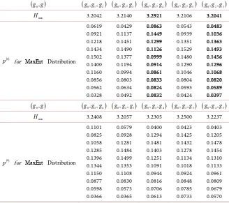
Table 7. Distributions of

(

MinMaxEnt ,

)

_m m=1,2,3,4.

t di ci pi

∗

(

)

1

MinMaxEnt

(

MinMaxEnt

)

2

(

MinMaxEnt

)

3

(

MinMaxEnt

)

4

[image:8.595.209.539.499.674.2]

1 5 0 0.0485 0.1269 0.0483 0.0489 0.0475 2 10 1 0.1068 0.1249 0.1036 0.1034 0.1217 3 12 5 0.1650 0.1210 0.1363 0.1314 0.1192 4 8 2 0.0971 0.1153 0.1493 0.1458 0.1292 5 10 0 0.0971 0.1081 0.1456 0.1466 0.1422 6 15 6 0.2039 0.0997 0.1296 0.1342 0.1421 7 9 3 0.1165 0.0905 0.1068 0.1117 0.1225 8 8 1 0.0874 0.0809 0.0820 0.0844 0.0898 9 4 0 0.0388 0.0711 0.0589 0.0578 0.0560 10 3 1 0.0388 0.0615 0.0397 0.0358 0.0298

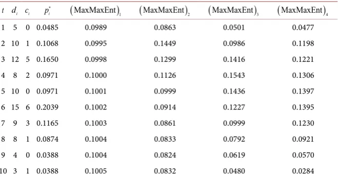
Table 8. Distributions of

(

MaxMaxEnt ,

)

_m m=1,2,3,4.

t di ci pi

∗

(

)

1

MaxMaxEnt

(

MaxMaxEnt

)

2

(

MaxMaxEnt

)

3

(

MaxMaxEnt

)

4

1 5 0 0.0485 0.0989 0.0863 0.0501 0.0477 2 10 1 0.1068 0.0995 0.1449 0.0986 0.1198 3 12 5 0.1650 0.0998 0.1299 0.1416 0.1221 4 8 2 0.0971 0.1000 0.1126 0.1543 0.1306 5 10 0 0.0971 0.1001 0.0999 0.1436 0.1397 6 15 6 0.2039 0.1002 0.0914 0.1227 0.1395 7 9 3 0.1165 0.1003 0.0861 0.0999 0.1230 8 8 1 0.0874 0.1004 0.0833 0.0792 0.0921 9 4 0 0.0388 0.1004 0.0824 0.0619 0.0570 10 3 1 0.0388 0.1005 0.0832 0.0480 0.0284

(9)

(

MinMaxEnt

)

₃ is more suitable and among of distributions

(

MaxMaxEnt

)

_m,

(

m

=

1,2,3,4

)

_{the distribution}

(

MaxMaxEnt

)

₄ is more convenient for statis-tical data. These results are also corroborated by graphical representation (see

Figures 1-4). Consequently, we shall consider Probability Density Function

( )

ˆ

f t , Cumulative Distribution Function F tˆ

( )

, Survival Function S tˆ

( )

and Hazard Rate h tˆ

( )

for only

(

MinMaxEnt

)

₃ and

(

MaxMaxEnt

)

₄ distributions. Although the distribution with the largest number of moment functions tends to fit better, it should be noted that in some cases, the set of moment functions with fewer elements is more informative then a different set of moment func-tions with more number of elements.

Table 9. The obtained results for

(

MinMaxEnt

)

_m, m=1,2,3,4.

Distribution of MinMaxEnt H Calculated value of _Chi-Square _{Chi-Square value}Probability of Table value of _{Chi-Square RMSE}

(

MinMaxEnt

)

1 3.2854 4.4310 0.8163

2 8,α 15.51

χ = 0.3158

(

MinMaxEnt

)

2 3.2041 0.6512 0.9987

2 7,α 14.07

χ = _0.1873

(

MinMaxEnt

)

3 3.2000 1.7787 0.9389

2 6,α 12.59

χ = 0.1799

(

MinMaxEnt

)

4 3.1932 1.6161 0.8993

2 5,α 11.07

χ = 0.1830

Table 10. The obtained results for

(

MaxMaxEnt

)

_m, m=1,2,3,4.

Distribution of MinMaxEnt H Calculated value of _Chi-Square _{Chi-Square value}Probability of Table value of _{Chi-Square RMSE}

(

MaxMaxEnt

)

1 3.3219 5.3820 0.7161

2 8,α 15.51

χ = 0.3492

(

MaxMaxEnt

)

2 3.2921 4.9233 0.6693

2 7,α 14.07

χ = 0.3492

(

MaxMaxEnt

)

3 3.2155 2.2804 0.8922

2 6,α 12.59

χ = 0.2104

(

MaxMaxEnt

)

4 3.1937 1.6383 0.8966

2 5,α 11.07

χ = 0.1888

(a) (b)

[image:9.595.206.540.260.358.2] [image:9.595.140.538.400.708.2]

(10)

[image:10.595.140.537.60.259.2]

(a) (b)

Figure 2. Graphic of

(

MinMaxEnt

)

2 and

(

MaxMaxEnt

)

2 distributions.

[image:10.595.138.537.292.485.2]

(a) (b)

Figure 3. Graphic of

(

MinMaxEnt

)

3 and

(

MaxMaxEnt

)

3 distributions.

(a) (b)

[image:10.595.140.538.520.708.2]

(11)

4.2. Availability of GEOD to Survival Data in the Sense of Shannon

Measure

In order to establish availability of GEOD to survival data in the sense of Shan-non measure it is required to consider entropy values of GEOD.

From Table 3 it is seen that the MinMaxEnt (the MaxMaxEnt) distribu-tion is realized by vector funcdistribu-tion

(

)

( )

2

(

) (

)

0, 2 1, 0, 3 1,ln

g g = x g g = x _and

(

)

(

MinMaxEnt ₁

)

3.2854

(

MaxMaxEnt

)

₁

)

3.3219

)

H = H = .

(

)

(

2

)

(

)

(

( )

2

)

0, ,2 3 1, ,ln 0, ,1 4 1, , ln

g g g = x x g g g = x x _and

(

)

(

MinMaxEnt ₂

)

3.2041

(

MaxMaxEnt

)

₂

)

3.2921

)

H = H = .

(

)

(

2

(

)

2

)

(

)

(

2

(

2

)

0, , ,1 2 4 1, , , ln 0, , ,2 3 5 1, ,ln ,ln 1

g g g g = x x x g g g g = x x +x _and

(

)

(

MinMaxEnt ₃

)

3.2000

(

MaxMaxEnt

)

₃

)

3.2155

)

H = H = .

(

)

(

( )

2

(

2

)

(

)

(

2

( )

2

)

0, ,1 3, 4, 5 1, ,ln , ln ,ln 1 0, ,1 2, 3, 4 1, , ,ln , ln

g g g g g = x x x +x g g g g g = x x x x

and H

(

MinMaxEnt

)

₄

)

=3.1932

(

H

(

MaxMaxEnt

)

₄

)

=3.1937

)

.

Comparison of GEOD with each other in the sense of Shannon measure shows that along of these distributions

(

MinMaxEnt

)

₄ is better.

The results of our investigation according to using known characterizing moment vector functions from K0,m are summarised in the form of following

Corollary.

Corollary 1. If by

(

MaxMaxEnt

) (

_m

(

MinMaxEnt

)

_m

)

denote the

MaxMaxEnt (the MinMaxEnt) distribution corresponding to m moment conditions generated by moment functions

g x g K

( )

,

∈

0,m, then inequality

(

)

(

)

(

)

(

)

(

)

(

)

(

11 22

)

MaxMaxEnt MaxMaxEnt

MinMaxEnt MinMaxEnt

m m

H H

>

is fulfilled, when m m1< 2. In other words, entropy value of the MaxMaxEnt

(the MinMaxEnt) distribution depending on the number m of moment con-ditions decreases.

Moreover for any m the inequality

(

)

(

MaxMaxEnt _m

)

(

MinMaxEnt

)

_m

)

H >H

takes place.

4.3. Availability of GEOD to Survival Data in the Sense of

Kullback-Leibler Measure

Now, we calculate the distance between observed distribution

(

1

, , ,

2 10

)

i

p

=

p p



p

given in Table 2 and distributions

( )

₍

₎

( )

₍

₎

mini MinMaxEnt ,i maxi MaxMaxEnt ,i 1, 2,3, 4

p = p = i= given in Table 7 and

(12)

It is known that the Kullback – Leibler distance between distributions

(

1

, , ,

2 n

)

p

=

p p



p

and

q

=

(

q q

1

, , ,

2



q

n

)

is obtained by formula

(

;

)

n₁ ln i i i

i p D p q p

q

=

∑

_.

By starting these formula Kullback-Leibler measures for the distance between observed distribution

p

i

=

(

p p

1

, , ,

2



p

10

)

and distributions

( )

₍

₎

( )

₍

₎

mini MinMaxEnt ,i maxi MaxMaxEnt ,i 1, 2,3, 4

p = p = i= are given in Table 11

and Table 12 respectively.

From Table 11 and Table 12 follows that along of GEOD

(

MinMaxEnt

)

₄ is better in the sense of Kullback-Leibler measure.

The results of our investigation according to using known characterizing moment vector functions from K0,m are summarised in the form of following

Corollary.

Corollary 2. If

p

i

=

(

p p

1

, , ,

2



p

10

)

observed distribution and

( )

₍

₎

(

( )

₍

₎

)

mini MinMaxEnt ,i 1, 2,3, 4 maxi MaxMaxEnt ,i 1, 2,3, 4

p = i= p = i= denote the

MinMaxEnt (the MaxMaxEnt ) distribution corresponding to i moment conditions generated by moment functions

g x g K

( )

,

∈

0,m, then inequality

( )

(

)

(

( )

)

( )

(

)

(

( )

)

(

)

1 2

min min

max max

; ;

m m

i i

m m

i i

D p p D p p

D p p D p p >

>

is fulfilled, when m m1< 2. In other words, Kullback-Leibler value of the

MinMaxEnt (the MaxMaxEnt) distribution depending on the number

m

of

moment conditions decreases.

Moreover for any i the inequality

( )

(

)

(

( )

)

maxi ; i mini ; i

D p p >D p p

[image:12.595.207.539.525.611.2]

takes place.

Table 11. Kullback-Leibler measure of

(

MinMaxEnt , 1,2,3,4

)

_m i= distributions.

(

MinMaxEnt , 1,2,3,4

)

_m i= distributions

(

( )

)

min; , 1,2,3,4 i

i

D p p i=

(

MinMaxEnt

)

1 0.3938

(

MinMaxEnt

)

2 0.3348

(

MinMaxEnt

)

3 0.3300

(

MinMaxEnt

)

4 0.3193

Table 12. Kullback-Leibler measure of

(

MaxMaxEnt , 1,2,3,4

)

_m i= distributions.

(

MaxMaxEnt , 1,2,3,4

)

_m i= distributions

(

( )

)

max; , 1,2,3,4 i

i

D p p i=

(

MaxMaxEnt

)

1 0.4441

(

MaxMaxEnt

)

2 0.4009

(

MaxMaxEnt

)

3 0.3457

[image:12.595.205.539.648.734.2]

(13)

4.4. Survival Expression of Distributions

(

MinMaxEnt

)

₃

,

(

MaxMaxEnt

)

₄

In this section survival data analysis is conducted by

(

MinMaxEnt

) (

₃

(

MaxMaxEnt

)

₄

)

distribution since the above acquired investi-gations

(

MinMaxEnt

) (

₃

(

MaxMaxEnt

)

₄

)

is more presentable for survival data among

(

MinMaxEnt

) (

_m

(

MaxMaxEnt

)

_m

)

, m=1, 2, , 4 distributions.

(

MinMaxEnt

)

₃ and

(

MaxMaxEnt

)

₄ estimations of Probability Density Function f tˆ

( )

, Cumulative Distribution Function F tˆ

( )

, Survival Function

( )

ˆ

S t and Hazard Rate h tˆ

( )

are given in Table 13 & Table 14, respectively. On basis of the results given in Table 13 & Table 14, graphs of f t F tˆ

( )

, ˆ

( )

,

( )

ˆ

[image:13.595.208.541.290.495.2]

S t and h tˆ

( )

are demonstrated in Figures 5(a)-(c) & Figures 6(a)-(c).

Table 13. Survival analysis by

(

MinMaxEnt

)

3.

t ni di ci f tˆ( ) (= MinMaxEnt)3 F tˆ( ) S tˆ( ) ( )

( ) ( )

ˆ ˆ

ˆ

f t h t

S t

=

1 200 5 0 0.0489 0.0489 0.9511 0.0514 2 195 10 1 0.1034 0.1523 0.8477 0.1220 3 184 12 5 0.1314 0.2837 0.7163 0.1834 4 167 8 2 0.1458 0.4295 0.5705 0.2556 5 157 10 0 0.1466 0.5761 0.4239 0.3458 6 147 15 6 0.1342 0.7103 0.2897 0.4632 7 126 9 3 0.1117 0.8220 0.1780 0.6275 8 114 8 1 0.0844 0.9064 0.0936 0.9017 9 105 4 0 0.0578 0.9642 0.0358 1.6145 10 101 3 1 0.0358 1.0000 0.0000 --

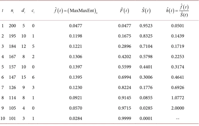
Table 14. Survival analysis by

(

MaxMaxEnt

)

4.

t ni di ci f tˆ( ) (= MaxMaxEnt)4 F tˆ( ) S tˆ( ) ( )

( )

ˆ ˆ

ˆ( )

f t h t

S t

=

[image:13.595.209.539.528.736.2]

(14)

(a) (b)

[image:14.595.168.535.61.522.2]

(c)

Figure 5. Survival expression of distribution

(

MinMaxEnt

)

₃.

5. Conclusion

(15)

(a) (b)

[image:15.595.168.539.61.556.2]

(c)

Figure 6. Survival expression of distribution

(

MaxMaxEnt

)

4.

is showed that,

(

MinMaxEnt

) (

3

(

MaxMaxEnt

)

4

)

is more suitable for statistical

data among

(

MinMaxEnt ,

)

_m m=1, 2,3, 4 MaxMaxEnt ,

(

)

_m m=1, 2,3, 4

)

. More-over,

(

MinMaxEnt

)

₃ is better for statistical data than

(

MaxMaxEnt

)

₄ in the sense of RMSE criteria. According to obtained distribution

(

MinMaxEnt

)

₃

(

)

(

MaxMaxEnt 4

)

estimator of Probability Density Function f tˆ

( )

, Cumulative

(16)

References

[1] Shamilov, A. (2006) A Development of Entropy Optimization Methods. Wseas Transactions on Mathematics, 5, 568-575.

[2] Shamilov, A. (2007) Generalized Entropy Optimization Problems and the Existence of Their Solutions. Physica A: Statistical Mechanics and Its Applications, 382, 465- 472. https://doi.org/10.1016/j.physa.2007.04.014

[3] Kaminski, D. and Geisler, C. (2012) Survival Analysis of Faculty Retention in Science and Engineering by Gender. Science, 335, 864-866.

https://doi.org/10.1126/science.1214844

[4] Reingold, E.M., Reichle, E.D. and Glaholt, M.G. (2012) Heather Sheridan, Direct Lexical Control of Eye Movements in Reading: Evidence from a Survival Analysis of Fixation Durations. Cognitive Psychology, 65, 177-206.

[5] Wang, H. and Dai, H.S. (2012) Accelerated Failure Time Models for Censored Sur-vival Data under Referral Bias. Biostatistics, 14, 313-326.

[6] Ebrahimi, N. (2000) The Maximum Entropy Method for Lifetime Distributions. Sankhyā: The Indian Journal of Statistics, Series A, 62, 236-243.

[7] Guyot, P., Ades, A., Ouwens, M.J. and Welton, N.J. (2012) Enhanced Secondary Analysis of Survival Data: Reconstructing the Data from Published Kaplan-Meier Survival Curves. BMC Medical Research Methodology, 12, 9.

https://doi.org/10.1186/1471-2288-12-9

[8] Joly, P., Gerds, T.A., Qvist, V., Commenges, D. and Keiding, N. (2012) Estimating Survival of Dental Fillings on the Basis of Interval-Censored Data and Multi-State Models. Statistics in Medicine, 31, 11-12.

[9] Lee, E.T. and Wang, J.W. (2003) Statistical Methods for Survival Data Analysis. Wi-ley-Interscience, Oklahoma.

[10] Deshpande, J.V. and Purohit, S.G. (2005) Life Time Data: Statistical Models and Methods, Series on Quality. Vol. 11, Reliability and Engineering Statistics, India. [11] Kapur, J.N. (1992) Kesavan, Entropy Optimization Principles with Applications. [12] Shamilov, A. (2009) Entropy, Information and Entropy Optimization. T.C. Anadolu

University Publication, Eskisehir.

[13] Shamilov, A. (2010) Generalized Entropy Optimization Problems with Finite Mo-ment Functions Sets. Journal of Statistics and Management Systems, 13, 595-603. https://doi.org/10.1080/09720510.2010.10701489

(17)

Submit or recommend next manuscript to SCIRP and we will provide best service for you:

Accepting pre-submission inquiries through Email, Facebook, LinkedIn, Twitter, etc. A wide selection of journals (inclusive of 9 subjects, more than 200 journals)

Providing 24-hour high-quality service User-friendly online submission system Fair and swift peer-review system

Efficient typesetting and proofreading procedure

Display of the result of downloads and visits, as well as the number of cited articles Maximum dissemination of your research work

Submit your manuscript at: http://papersubmission.scirp.org/