An improved framework for the inverse analysis of skeletal muscle tissue in vivo

An Improved Framework for the

Inverse Analysis of Skeletal Muscle

Tissue

In-Vivo

An Improved Framework for the

Inverse Analysis of Skeletal

Muscle Tissue In-Vivo

Kevin Mattheus Moerman

A thesis submitted to the University of Dublin, Trinity College, in partial fulfilment

of the requirements for the degree of

Doctor in Philosophy

An Improved Framework for the

Inverse Analysis of Skeletal Muscle

Tissue

In-Vivo

Kevin Mattheus Moerman, M.Sc. B.Eng.

A thesis submitted to the University of Dublin Trinity College, in partial fulfilment of the requirements for the degree of

Doctor in Philosophy

Trinity College Dublin April 2012

Supervisor:

Dr. Ciaran K. Simms1

Internal Examiner:

Prof. Daniel J. Kelly1

External Examiner:

Prof. Cees W.J. Oomens2

1_{Trinity Centre for Bioengineering, University of Dublin, Trinity College, Dublin, Ireland}

I

-Declaration

I declare that this thesis has not been submitted as an exercise for a degree at this or any other university and it is, unless otherwise referenced, entirely my own work.

I agree to deposit this thesis in the University’s open access institutional repository or allow the library to do so on my behalf, subject to Irish Copyright Legislation and Trinity College Library conditions of use and acknowledgement.

Kevin Mattheus Moerman

II

-Summary

This thesis focusses on the development of an experimental and computational framework for the non-invasive analysis of the passive mechanical properties of living human skeletal muscle tissue. This is relevant to many areas of research including impact biomechanics and rehabilitation engineering.

Although constitutive models have been proposed for muscle tissue these have been insufficiently validated for human tissue which requires non-invasive methods. Non-invasive analysis of the mechanical properties of soft tissue requires non-invasive mechanical exciting and inverse analysis of non-invasively measured experimental boundary conditions such as tissue deformation and applied load.

Magnetic Resonance Imaging (MRI) provides excellent soft tissue contrast without ionizing radiation. In addition it allows for the measurement of soft tissue anatomy, architecture and deformation boundary conditions. Hence for mechanical excitation a novel MRI compatible and computer controllable soft tissue indentation device was developed and implemented with an accurate high acquisition rate (100Hz) optical force sensor capable of viscoelastic force registration.

In order to measure the resultant deformation SPAtial Modulation of the Magnetisation (SPAMM) tagged MRI was used. Traditional SPAMM tagging methods require large numbers of repetitions of motion cycles causing repeatability difficulties and volunteer discomfort. However for this thesis a unique set of high speed SPAMM tagged MRI techniques, and fully automatic post-processing methods based on Gabor wavelet filtering, were developed allowing for the measurement of complex dynamic 3D deformation following the combination of just 3 motion cycles. The SPAMM tagged MRI techniques were validated using marker tracking in a silicone gel phantom and underwent in-vivo evaluation whereby sub-voxel accuracy and precision levels were reported.

III

-Finally an FE modelling framework was presented whereby detailed anatomically accurate 3D FE models can be generated from anatomical MRI and where diffusion tensor MRI based fibre directions could be incorporated as well.

A bank of experimental data was created for MRI based volunteer upper arm indentation for use in future biomechanical studies consisting of anatomical and diffusion tensor MRI data, 3D displacement vector fields and indentation force data.

V

VII

-Acknowledgements

First of all I would like to thank Dr. Ciaran Simms (Trinity College Dublin) for his fantastic role as my supervisor! I don’t think I could imagine a better supervisor, always there, always positive, always motivating. Thanks for being so incredibly patient with me and for trusting me and allowing me to explore tangents sometimes and for steering me back into the right direction other times. Thanks Ciaran, and also my Principal Investigator Dr Caitríona Lally (Dublin City University) for this fantastic opportunity!

Thanks also to my colleague Vittoria Flamini at Dublin City University for our collaboration early on in the project. I would also like to thank my colleagues at the Trinity Centre for Bioengineering for the nice working atmosphere. Thanks especially to Thomas Nagel for coffees and walks around campus while discussing continuum mechanics when I was in Dublin and later over Skype when I was in Amsterdam. Thanks also to Michael Takaza and Dr. Melanie van Loocke for sharing their experimental data with me.

I am also grateful to Dr. Aart Nederveen and Drs. Andre Sprengers at the Academic Medical Centre, Amsterdam. Thanks for the very fruitful collaboration in relation to MRI. Also, Aart thank you for effectively co-supervising me on the MRI side of things and for financially adopting me after my third year and allowing me to work at the AMC! I would like to thank all colleagues at the AMC. Especially Andre Sprengers for advice on SPAMM tagged MRI and for joining me even on Sundays or in the middle of the night if required for some more MRI scanning! Thanks also for advice on the implementation of scale-space methods for SPAMM tagged MRI analysis. I’m also grateful to Dr. Matthan Caan (Matlab advice), Martijn Froeling (assistance for diffusion tensor MRI) and Paul Groot (advice on the TTL triggering system and help compiling the customized FEBio source codes).

Thanks to Prof. Sam Evans and Dr. Cathy Holt (Cardiff University Wales) for the collaboration in relation to DIC and Sam for introducing me to FEBio.

I would also like to thank Prof. Gerard Ateshian and Dr. Steve Maas for their often extensive replies to my FEBio queries posted on the FEBio forum.

VIII

-Thanks also to my dear friends and former housemates while in Dublin Dr. Brendan Holland and Dr. Daniel Isemann. Thanks for always being there to discuss difficulties with my project or for pure procrastination and the many hours spend on Trinity’s croquet lawn.

I also thank my parents and family for always supporting me.

Lastly I am eternally grateful to my dearest wife Elizabeth! Thanks for the never ending support and your enormous patience! Thanks for listening whenever I went on and on about bubble membranes, Gabor wavelets and Bucky-balls. Isaac thanks also to you also for giving me something amazing to look forward to and thank you for granting me a reasonable amount of sleep during your first weeks on this world so that I felt fit enough to get this thesis finished.

IX

-Table of

Contents

DECLARATION ... I

SUMMARY ... II

ACKNOWLEDGEMENTS ... VII

LIST OF PUBLICATION RESULTING FROM THIS STUDY ... XIV

Journal papers XIV

Co-authored journal papers XIV Conference proceedings XV

NOMENCLATURE ... XVII

Mathematical notation XVII Symbols XVII

Abbreviations XX

1 INTRODUCTION ... 1

1.1 RATIONALE OF THE STUDY ... 1

1.2 OBJECTIVES OF THE STUDY ... 3

1.3 OUTLINE OF THE THESIS ... 4

2 THEORETICAL FRAMEWORK ... 7

2.1 INTRODUCTION ... 8

2.2 BASICS OF CONTINUUM MECHANICS ... 8

2.2.1 Introduction 8 2.2.2 Vector and tensor algebra 8 2.2.3 The continuum hypothesis 14 2.2.4 Motion 14 2.2.5 Deformation 15 2.2.6 Stretch and rotation 16 2.2.7 Strain 18 2.2.8 Stress 19 2.2.9 Strain energy 21 2.2.10 Constitutive equations 22 2.2.11 Modelling anisotropy 26 2.2.12 Viscoelasticity 29 2.3 BASICS OF MAGNETIC RESONANCE IMAGING ... 34

2.3.1 Introduction 34

2.3.2 Angular momenta and magnetic moments 34 2.3.3 Equilibrium alignment of spin 36

2.3.4 Dynamic equilibrium 37

2.3.5 Alteration of dynamic equilibrium 39 2.3.6 Relaxation to dynamic equilibrium 39

X

-2.3.8 Position encoding 42

2.3.9 Anatomical magnetic resonance imaging 44

2.3.10 MRI techniques based on motion induced phase shifts 45 2.3.11 Tagged Magnetic Resonance Imaging 49

2.4 BASICS OF IMAGE PROCESSING ... 52

2.4.1 Introduction 52 2.4.2 Background on image data 52 2.4.3 Segmentation and filtering 54 2.4.4 Spatial transformations 56 2.4.5 Image correlation and registration 57 3 LITERATURE REVIEW ... 60

3.1 INTRODUCTION ... 60

3.2 SKELETAL MUSCLE ANATOMY AND PHYSIOLOGY ... 61

3.2.1 Introduction 61 3.2.2 Skeletal muscle tissue architecture 61 3.2.3 Muscle tone and passive stiffness enhancement 64 3.2.4 Muscle fibre type, distribution and orientation 65 3.2.5 Conclusions 66 3.3 SKELETAL MUSCLE TISSUE MECHANICAL BEHAVIOUR ... 67

3.3.1 Introduction 67 3.3.2 Invasive mechanical property assessment and analysis of excised tissue samples 67 3.3.3 Non-invasive mechanical property assessment 77 3.3.4 Comments on constitutive modelling of skeletal muscle tissue 83 3.3.5 Conclusions 85 3.4 NON-INVASIVE IMAGING MODALITIES ... 87

3.5 MRI COMPATIBLE ACTUATOR AND SENSOR DEVICES ... 87

3.6 MRI BASED MEASUREMENT OF SOFT TISSUE DEFORMATION ... 90

3.7 VALIDATION OF MRI DERIVED MOTION AND DEFORMATION ... 91

3.8 SUMMARY AND PROPOSED APPROACH ... 92

4 STUDY I A NOVEL MRI COMPATIBLE SOFT TISSUE INDENTOR AND OPTICAL FIBRE BRAGG GRATING FORCE SENSOR ... 97

4.1 INTRODUCTION ... 98

4.2 METHODS ... 98

4.2.1 Fibre Bragg Grating Based optical force sensing 99 4.2.2 The soft tissue indentor system 100 4.2.2.1 THE MRI COMPATIBLE SOFT TISSUE INDENTOR ASSEMBLY ... 100

4.2.2.2 THE MRI ACTUATOR ASSEMBLY ... 101

4.2.2.3 THE INDENTOR HEAD AND FORCE SENSOR ASSEMBLY ... 102

4.2.2.4 ACTUATOR MOTION CONTROL AND DATA ACQUISITION ... 103

4.2.3 Optical force sensor calibration 104 4.2.4 Evaluation of the indentor system performance 105 4.2.4.3 EVALUATION OF THE SYSTEM MRI COMPATIBILITY... 108

4.3 RESULTS ... 109

XI

-4.4 DISCUSSION ... 115

4.5 CONCLUSIONS ... 120

5 STUDY II DIC AND INVERSE FEA FOR THE DETERMINATION OF THE MECHANICAL PROPERTIES OF SOFT TISSUE ... 122

5.1 INTRODUCTION ... 123

5.2 METHODS ... 123

5.3 RESULTS ... 125

5.4 DISCUSSION AND CONCLUSIONS ... 128

6 STUDY III A VALIDATION FRAMEWORK FOR MRI BASED DEFORMATION MEASUREMENT ... 130

6.1 INTRODUCTION ... 131

6.1.1 The tissue phantom 131 6.1.2 MR Imaging 132 6.1.3 Marker tracking method 132 6.1.4 Evaluation of marker tracking method using simulated magnitude MR image data 135 6.1.5 Simulation of a noiseless image and analysis of geometric bias 136 6.1.6 Simulation of noisy magnitude MR data and analysis of the noise effects 140 6.2 RESULTS ... 141

6.2.1 Evaluation of the geometric bias in the marker tracking method 142 6.2.2 Evaluation of the performance on the marker tracking method in the presence of noise. 143 6.3 DISCUSSION ... 144

6.4 CONCLUSIONS ... 144

7 STUDY IV THE MRI BASED MEASUREMENT OF STATIC 3D SOFT TISSUE DEFORMATION ... 146

7.1 INTRODUCTION ... 147

7.2 METHODS ... 148

7.2.1 MRI sequence design 148 7.2.2 The validation set-up: indentor and soft tissue phantom 152 7.2.3 Deriving tissue deformation from the SPAMM tagged MRI data 153 7.2.4 Analysis of precision and accuracy 158 7.3 RESULTS ... 159

7.3.1 Precision of tag point location 159 7.3.2 Precision of displacement magnitude 160 7.3.3 Accuracy of displacement measurement in the phantom 162 7.4 DISCUSSION ... 163

7.5 CONCLUSIONS ... 166

8 STUDY V THE MRI BASED MEASUREMENT OF DYNAMIC 3D SOFT TISSUE DEFORMATION ... 168

8.1 INTRODUCTION ... 169

8.2 METHODS ... 170

8.2.1 The experimental set-up: indentor and soft tissue phantom 170 8.2.2 MRI sequence 171 8.2.3 Spatial characteristics of SPAMM tags 174 8.2.4 Deriving tissue deformation from the SPAMM tagged MRI data 176 8.2.5 Analysis of precision and accuracy 186 8.3 RESULTS ... 187

XII

-8.3.2 Precision of individual dynamic displacement 189 8.3.3 Accuracy of cumulative dynamic displacement 190 8.3.4 Accuracy of displacement in the phantom 192

8.4 DISCUSSION ... 193

8.5 CONCLUSIONS ... 196

STUDY VI CONSTITUTIVE MODELLING OF SKELETAL MUSCLE TISSUE ... 198

8.6 INTRODUCTION ... 199

8.7 METHODS ... 200

8.7.1 The anisotropic and non-linear elastic properties of muscle tissue 200 8.7.2 Constitutive modelling of non-linear elasticity 204 8.7.3 Modelling of volumetric tension compression non-linearity 213 8.7.4 Inverse FEA based constitutive model evaluation 213 8.8 RESULTS ... 216

8.8.1 Isotropic Ogden hyperelastic (ISO) 216 8.8.2 Fibre reinforced transversely isotropic Ogden hyperelastic (TISO) 217 8.8.3 Orthotropic fibre family reinforced Ogden (TCNL) model for compression 219 8.8.4 Ellipsoidal fibre distribution (EFD) models for tension and compression 220 8.8.5 Gaussian Modulated Spherical Fibre Distribution Ogden hyperelastic (GMSFD) model for tension and compression 223 8.8.6 Modelling of volumetric tension compression non-linearity 226 8.9 DISCUSSION ... 226

8.10 CONCLUSIONS ... 228

9 STUDY VII MRI BASED DERIVATION OF DETAILED FINITE ELEMENT MODELS INCORPORATING FIBRE ARCHITECTURE ... 229

9.1 INTRODUCTION ... 230

9.2 METHODS ... 230

9.2.1 MRI based indentation experiments 230 9.2.2 FE model construction 231 9.2.3 Iterative inverse FEA based optimisation 235 9.3 RESULTS ... 235

9.4 DISCUSSION ... 236

9.5 CONCLUSIONS ... 236

10 DISCUSSION, CONCLUSIONS AND FUTURE WORK ... 237

XIV

-List of publication resulting from this

study

Journal papers

• Moerman, K.M., Holt, C.A., Evans, S.L. and Simms, C.K., "Digital image correlation and finite element modelling as a method to determine mechanical properties of human soft tissue in vivo", Journal of Biomechanics 42, 1150-1153 (2009).

• Moerman, K.M., Kerskens, C.M., Lally, C., Flamini, V. and Simms, C.K., "Evaluation of a Validation Method for MR Imaging-Based Motion Tracking Using Image Simulation", EURASIP Journal on Advances in Signal Processing 2010, 11 pages (2010).

• Moerman, K.M., Sprengers, A.M., Simms, C.K., Lamerichs, R.M., Stoker, J. and Nederveen, A.J., "Validation of SPAMM tagged MRI based measurement of 3D soft tissue deformation", Medical Physics 38, 13 (2011).

• Moerman, K.M., Sprengers, A.M., Simms, C.K., Lamerichs, R.M., Stoker, J. and Nederveen, A.J., "Validation of Continuously Tagged MRI for the Measurement of Dynamic 3D Soft Tissue Deformation", Medical Physics 39, 1793-1810, (2012).

• Moerman, K.M., Sprengers, A.M.J., Nederveen, A.J. and Simms, C.K., "A Novel MRI Compatible Soft Tissue Indentor and Fibre Bragg Grating Force Sensor", Medical Engineering & Physics Article in review (2012).

Co-authored journal papers

• Flamini, V., Kerskens, C.M., Moerman, K.M., Simms, C.K. and Lally, C., "Imaging Arterial Fibres Using Diffusion Tensor Imaging—Feasibility Study and Preliminary Results", EURASIP Journal on Advances in Signal Processing 2010, 13 (2010).

XV

-Conference proceedings

• K.M. Moerman and C.K. Simms, “Non-invasive determination of soft tissue deformation using tagged MRI: application to a silicone phantom”, Bioengineering in Ireland, 2008.

• K.M. Moerman and C.K. Simms, “A Validation Method for Motion Tracking Techniques Based on Tagged MRI”, Bioengineering in Ireland, 2009.

• K.M. Moerman, C. Lally, C.K. Simms, “A 3D Image Object tracking Algorithm Based on Sparse Masking and Adjacency Analysis”, The 10th _{United States National} Congress of Computational Mechanics, (Columbus, OHIO, 2009)

• K.M. Moerman, A. M. Sprengers, A. J. Nederveen, C.K. Simms, “Towards the Non-Invasive Determination of the Mechanical Properties of Living Human Soft Tissue”, Bioengineering in Ireland, 2010.

• K. M. Moerman, A. M. Sprengers, A. J. Nederveen, C. A. Holt, S. L. Evans, C. Lally and C. K. Simms, "Non-Invasive Imaging and Inverse Finite Element Analysis for the Determination of the Mechanical Properties of Soft Tissue," in Computational Methods in Biomechanics Biomedical Engineering, (Valencia, Spain, 2010).

• K. M. Moerman, C. K. Simms, A. M. Sprengers and A. J. Nederveen, "Experimental Validation of SPAMM Tagged Magnetic Resonance Imaging Based Measurement of Non-uniform 3D Soft Tissue Deformation," in ISMRM ESMRMB Joint Annual Meeting, (Stockholm, Sweden, 2010).

• K. M. Moerman, A. M. Sprengers, A. J. Nederveen and C. K. Simms, "Non-invasive Measurement of 3D Soft Tissue Deformation and Force: Application to Indentation Tests on the Human Upper Arm," in 17th Congress of the European Society of Biomechanics, (Edinburgh, 2010).

• K. M. Moerman and C. K. Simms, "A novel MRI compatible Soft Tissue Indentor and Fibre Bragg Grating Force Sensor " in Fourth European Workshop on Optical Fibre Sensors, Vol. 7653, edited by J. L. Santos, B. Culshaw, J. M. López-Higuera and W. N. MacPherson (SPIE, Porto, Portugal, 2010).

XVI

-• K. M. Moerman, A. M. Sprengers, C. K. Simms, A. E. Bohte, R. Lamerichs, R. Sinkus and A. J. Nederveen, "Combined MRE and SPAMM tagged MRI for the analysis of large strain soft tissue mechanical properties " in ISMRM ESMRMB Joint Annual Meeting, (Montreal, 2011).

XVII

-Nomenclature

Mathematical notation

Notation Description

𝑎,𝛼,𝑏,𝛽 Scalars

𝐚 Vector

|𝐚| Magnitude of vector 𝐚

𝐚 ∙ 𝐛 The dot (or scalar or inner) product of the vectors 𝐚 and 𝐛 𝐚×𝐛 The cross (or vector or outer) product of the vectors 𝐚 and 𝐛

𝐚⨂𝐛 The dyad (or tensor) product of the vectors 𝐚 and 𝐛

𝐀 A (second-order unless otherwise stated) tensor or matrix

𝐴𝑖𝑗 Element i, j of tensor 𝐀

𝐀 ∶ 𝐁 The double-dot contraction of tensors 𝐀 and B

𝐀−1 _{The inverse of tensor 𝐀}

𝐀T _{The transpose of tensor 𝐀}

tr(𝐀) The trace of tensor 𝐀

det(𝐀) The determinant of tensor 𝐀

dev(𝐀) The deviatoric of tensor 𝐀 Δ𝐚 The gradient of 𝐚

∇𝑥𝐚 The gradient of 𝐚, defined as ∂ai

∂xi

𝜆̃ Modified variable 𝜆 𝐈 The identity tensor

𝟎 The zero tensor

𝐌 ∗ 𝐅 Convolution of 𝐌 and 𝐅 ℱ{𝐌} The Fourier transform of 𝐌

ℱ{𝐌}−1 _{The inverse Fourier transform of 𝐌}

Symbols

XVIII -Symbol Description

𝔼3 _{3D Euclidian space}

ℰ Right-handed orthonormal Cartesian basis in 𝔼3

𝐞𝑖 Orthonormal basis vectors

𝛿 The Kronecker Delta

Ω A continuum body

𝑃 A material point in Ω

𝑡 Time

𝒙 Position vector in Eulerian configuration

𝑿 Position vector in Lagrangian configuration

𝝌 Motion of material point

𝐮 Displacement vector

𝐅 Deformation gradient tensor

𝐃 Inverse of the deformation gradient tensor 𝐅

v, V Volume in the in Eulerian, Lagrangian configuration

𝐽 The Jacobian of the deformation gradient tensor (continuum mechanics) or angular momentum (MRI physics)

𝜆,𝜆𝑖 Stretch, a Lamé modulus (continuum mechanics), may also represent diffusion tensor Eigenvalue (MRI physics) or the reflected Bragg wavelength (physics of FBG sensors)

𝐐 The rotation tensor

𝐔 The left stretch tensor

𝐕 The right stretch tensor

𝐂 The right Cauchy-Green tensor

𝐁 The left Cauchy-Green or Finger tensor (continuum mechanics), External magnetic field (MRI physics)

𝐼𝑖 Deformation invariants

𝛆 The linear (Cauchy, Biot, small or infinitesimal) strain tensor

𝐄 The Green-Lagrange strain tensor

𝐇 The Logarithmic (or Hencky) strain tensor

𝑓,𝐹 Force, 𝑓may also refer to a function

XIX

-𝒏,𝑵 Surface normal vector in Eulerian, Lagrangian configuration

𝐭,𝐓 Traction vectors, in Eulerian, Lagrangian configuration (continuum mechanics), 𝐓 may also represent a spatial transformation tensor (image processing)

𝛔 The Cauchy or true stress tensor (continuum mechanics), standard deviation of Gaussian function (statistics, image processing)

𝐏 Piola-Kirchoff or Lagrangian stress tensor

𝐒 Second Piola-Kirchoff stress tensor (continuum mechanics), may also represent a deformation transformation tensor (image processing)

𝛕 Kirchoff stress tensor

𝒫𝑒𝑥𝑡 External mechanical power

𝒦 Kinetic energy

𝛱𝑖𝑛𝑡 Internal mechanical work

Ψ Strain-energy density (Helmholtz free-energy) function

λ A Lamé (material) parameter, or spring constant in rheological model

µ,µ𝑖 A Lamé material parameter, the shear modulus, a spring constant in rheological model, constant in (e.g. Ogden) hyperelastic

constitutive law E The Young’s modulus

𝜈 The Poisson’s ratio

𝜅 The bulk modulus

𝑐𝑖𝑗 Material constants in constitutive law

𝛼𝑖 Material constant in (e.g. Ogden) hyperelastic constitutive law

𝑛,𝑁 Population size or number of summation iterations, or number of spins in a voxel (MRI physics)

𝐀 Texture or structure tensor

𝐚 Fibre or texture direction vector

𝜉𝑖,𝜉 Fibre material parameter for tension-compression non-linear orthotropic and ellipsoidal/spherical fibre distribution models

XX

-orthotropic and ellipsoidal/spherical fibre distribution models. Alternatively this may refer to Criscione invariations

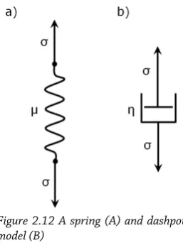
η Viscosity constant in rheological model

𝐺 Relaxation modulus (continuum mechanics). Magnetic field gradient (MRI physics).

𝜏𝑖 Viscoelastic material constant for discrete relaxation function

𝛾𝑖 Viscoelastic material constant for discrete relaxation function

𝑀 An image matrix (image processing)

𝑇1 Spin-lattice relaxation time

𝑇2 Spin-spin relaxation time

Abbreviations

Abbreviation Description

MR Magnetic Resonance

MRI Magnetic Resonance Imaging MRE Magnetic Resonance Elastography

SPAMM SPAtial Modulation of the Magnetisation CSPAMM Complementary SPAMM

PCMRI Phase Contrast MRI HARP Harmonice Phase

DENSE Displacement Encoding with Stimulated Echoes DTI Diffusion Tensor Imaging

DICOM Digital Imaging and Communication in Medicine FE Finite Element

FEA Finite Element Analysis FBG Fibre Bragg Grating

ACG Adjacency Coordinate Group OCV Object Central Voxel

PDF Probability Density Function SNR Signal to Noise Ratio

XXI -TTL Transistor-Transistor Logic

SSDM Sum of Squared Differences Matrix ECG Electrocardiogram

POM polyoxymethylene RMS Root Mean Square

SSQD Sum of Squared Differences ISO Isotropic Ogden hyperelastic

TISO Transversely Isotropic Ogden hyperelastic

TCNL Tension Compression Non-Linear Orthotropic Ogden hyperelastic

EFD Ellipsoidal Fibre Distribution

GMSFD Gaussian Modulation Spherical Fibre Distribution Ogden Hyperelastic

1

-1

INTRODUCTION

1.1

Rationale of the study

This thesis focusses on the development of an experimental and computational framework for the non-invasive analysis of the passive mechanical properties of skeletal muscle tissue. Of interest here is the development of methods to non-invasively analyse the non-linear and anisotropic elastic and viscoelastic properties of passive living skeletal muscle tissue.

The analysis of passive skeletal muscle soft tissue mechanical properties is relevant to many fields of research including the well-known applications to: impact biomechanics1-3_{, rehabilitation engineering}4-7_{, tissue engineering}8, 9_{, skeletal muscle}

behaviour simulation during gait10 _{and surgical simulation}11-14_{. Less well-known are the}

applications to the study of: soft tissue drug transport15, 16_{, extra-ocular muscle disorders} 17_{, oro-facial movements}18_{, and in zoology, caterpillar locomotion}19 _{and the simulation of}

squid tentacle strike to catch prey20_.

Experimental work on the mechanical properties of muscle tissue have largely focussed on excised tissue samples (e.g. for compression21 _{and tension}22_{) demonstrating}

skeletal muscle tissue to be non-linear, viscoelastic and anisotropic. Constitutive models have also been proposed (e.g.23, 24_{) however the anisotropic properties of such models}

have not been evaluated for multiple load directions. In addition, current constitutive modelling approaches model muscle tissue as reinforced in the fibre direction while recent experimental data21, 22 _{demonstrates that the transverse direction is most}

dominant. Hence appropriately validated models for anisotropy have not been presented to date.

Translation of constitutive property analysis to living human tissue presents with significant challenges and requires non-invasive methods. Apart from validation of constitutive models for living human tissue, non-invasive mechanical property analysis has many medical applications such as: lesion detection25 _{, pressure ulcer research}26, 27_{, to}

distinguish healthy and pathologic muscle28_{, or for the assessment of limb}

immobilisation and contracture29_{. However the non-invasive evaluation of detailed}

2

-and inverse analysis of detailed non-invasively measured experimental boundary conditions (including 3D tissue deformation and fibre architecture). Some authors have used indentation tests on skeletal muscle30, 31_{, but the tissue was then assumed to be}

isotropic and linear in elastic and viscoelastic properties. In addition elastography methods have been employed (using image based analysis of small strain wave propagations) for soft tissue. However elastography has only been applied to small strain measures and often linear elasticity is assumed (see review article32_{). In contrast,}

non-invasive imaging methods that allow detailed measurement of human soft tissue motion and deformation (due to known loading conditions), combined with inverse FEA allow for the evaluation of more complex and large strain constitutive models.

Magnetic resonance imaging (MRI) is an ideal modality for the non-invasive analysis of soft tissue biomechanics as it provides excellent soft tissue contrast without exposing subjects to ionizing radiation. In addition it allows for the measurement of various biomechanical boundary conditions required for inverse analysis of tissue properties, such as 3D tissue geometry (segmentable from anatomical MRI), 3D architecture (based on diffusion tensor MRI e.g.33_{) and accurate 3D soft tissue}

deformation measurement (e.g. based on tagged MRI, see review article34_).

Non-invasive mechanical excitation of tissue (e.g. indentation) for mechanical property analysis inside an MRI scanner requires accurate computer controllable and MRI compatible actuators and force sensors. Ensuring safety and compatibility of such systems is not trivial. Although MRI compatible actuators and force sensors have been developed for other applications such as MRI robotics (e.g.35, 36_{), MRI guided surgical}

interventions (e.g.37-39_{), MRI based catheterisation (e.g.}40_{), functional MRI (e.g.}41, 42_{) and}

the study of pressure ulcer development (e.g.43_{), to date no computer controlled MRI}

based actuator system suitable for human skeletal muscle tissue mechanical property investigation has been proposed.

Once mechanical excitation has been applied, MRI can be employed for the non-invasive measurement of 3D soft tissue deformation. MRI based methods to study soft tissue deformation of human soft tissue in-vivo is also relevant to many research areas; for instance, the analysis of organ and bowel motility44_{, the assessment of tumor}

motion45_{, the study of cardiac biomechanics}46 _{and preoperative planning}47_{. However}

3

-acquisitions requiring the combination of large numbers of motion cycles. This has confined the application of SPAMM tagged MRI to the analysis of highly repeatable and periodic movements and has mainly been applied to the heart46, 48, 49_{. Recently other}

tissue types have also been analysed for repeatedly induced motions of the tongue50 ₍₁₆

volunteer speech repetitions per slice), brain51 _{(144 volunteer rotational head}

accelerations) and eyes52 _{(>135 repeated left to right eye movements). For the purpose of}

mechanical indentation based mechanical property investigation these methods thus result in repeatability constraints and possible discomfort, highlighting the need to develop faster SPAMM techniques requiring a minimum of repeated motion cycles.

1.2

Objectives of the study

This thesis focusses on the development of a framework of computational and experimental methods for the non-invasive analysis of skeletal muscle tissue mechanical properties. Since MRI is the most suitable non-invasive modality and large strain is of interest, indentations will be applied during which force measurements are required, hence our first objective is:

1) To design and validate an MRI compatible soft tissue indentation system and force sensor

Since MRI based deformation measurement was challenging at the start of this thesis and required validation the second objective evaluates an alternative imaging method for deformation measurement combined with indentation and inverse FEA, namely digital image correlation (DIC), the second objective is thus:

2) To evaluate the indentation and inverse FEA based derivation of constitutive parameters based on DIC based deformation measurement.

The third objective for this thesis relates to the fact that MRI based motion measurement methods require validation:

3) To develop and evaluate methods to validate MRI derived soft tissue deformation. The fourth objective concerns the MRI based measurement of deformation during the indentation:

4

-The inverse FEA based constitutive parameter identification framework requires an appropriate starting constitutive model with initial parameters based on excised animal tissue data. This model needs to capture anisotropy for the transverse, longitudinal and intermediate direction responses. Hence the fifth objective was:

5) To develop a constitutive modelling framework capturing the anisotropic, non-linear and viscoelastic mechanical properties of skeletal muscle tissue.

Finally once an MRI compatible indentor has been used to apply indentation to a volunteer muscle site, force was measured using an MRI compatible force sensor and deformation was measured using SPAMM tagged MRI, one can start with the derivation of inverse FEA procedures for constitutive parameter identification. Thus the final objective was:

6) To develop methods to derive detailed anatomical models from MRI data incorporating fibre architecture allowing for the evaluation of tissue anisotropy.

1.3

Outline of the thesis

Theoretical framework

This chapter highlights: the theory of continuum mechanics, basics of MRI, and the basics of image processing.

Literature review

The following topics are discussed: the anatomy and physiology of skeletal muscle and its relation to the mechanical properties, experimental and computational modelling studies on the mechanical properties of skeletal muscle tissue, a brief discussion on non-invasive imaging modalities, MRI compatible actuators and sensor devices, MRI based measurement of soft tissue deformation and finally validation methods for MRI derived motion and deformation measurement.

5

-Study II: Digital Image Correlation and Finite Element Modelling as a Method to Determine Mechanical Properties of Soft Tissue

Since the development of MRI techniques was initially challenging study II evaluates the more straight-forward (but limited to surface measurements) alternative of DIC combined with inverse FEA for bulk material property assessment.

Study III: A Validation Framework for MRI Based Deformation Measurement

In order to validate MRI derived deformation measures study III describes a validation framework for MRI derived deformation measurement based on tracking of markers in a silicone gel phantom. A marker tracking algorithm is proposed and independently validated.

Study IV: The MRI Based Measurement of Static 3D Soft Tissue Deformation

This study introduces novel SPAMM tagged MRI techniques and semi-automatic post-processing methods for the derivation of 3D static deformation measurements following just 3 motion cycles.

Study V: The MRI Based Measurement of Dynamic 3D Soft Tissue Deformation

This study expands the SPAMM tagged MRI techniques for dynamic 3D deformation measurements following only 3 motion cycles. In addition a novel fully automatic methodology is presented.

Study VI: Constitutive Modelling of Skeletal Muscle Tissue

Using experimental data on uni-axial loading of muscle tissue for tension and compression at varying load angles, an array of common constitutive models is put to the test. It is demonstrated that current models do not accurately model anisotropy and tension compression non-linearity of muscle tissue and a novel constitutive model is proposed incorporating longitudinal and transverse fibrous contributions.

Study VII: MRI Based Derivation of Detailed Finite Element Models Incorporating Fibre Architecture

6

-incorporating skin, muscle and fat tissue and muscle fibre directions. Thus enabling the study of anisotropy.

Discussion, conclusions and future work

7

8

-2.1

Introduction

The current study involves constitutive modelling, finite element modelling and analysis, non-invasive imaging and digital image processing. In order to provide the reader with an understanding of the theory behind these areas, prior to presenting a review of the literature, this section discusses the basics of continuum mechanics, magnetic resonance imaging and digital image processing.

2.2

Basics of continuum mechanics

2.2.1

Introduction

This section describes the basics of vector and tensor algebra and continuum mechanics. For a more detailed discussion the reader is referred to specialised literature (e.g. on tensor algebra53 _{and continuum mechanics}54-59_).

2.2.2

Vector and tensor algebra

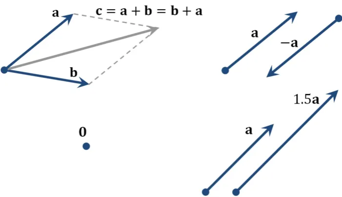
Physical quantities definable by a single real number are known as scalars and exhibit only magnitude. Vectors however are physical quantities with both direction and magnitude (in 3D vectors can be graphically represented by arrows as shown Figure 2.1). The magnitude (or length or norm) of a vector 𝐚 is denoted |𝐚| and is defined by:

|𝐚| = √𝐚 ⋅ 𝐚 2-1

A vector with a magnitude of 1 is called a unit vector. The dot (or inner or scalar) product of two vectors produces a scalar defined by:

𝐚 ∙ 𝐛 = |𝐚||𝐛| cos𝜃 2-2

with 𝜃 the angle between the two vectors. Two vectors are orthogonal if their dot product equals zero.

According to the parallelogram law when two vectors are added or subtracted a new vector is obtained (top left in Figure 2.1). A 3D Euclidean vector space can be defined, denoted by 𝔼3_{, where the following properties hold (see also Figure 2.1):}

𝐚+𝐛=𝐛+𝐚

(𝐚+𝐛) +𝐜=𝐚+ (𝐛+𝒄)

𝐚+𝟎=𝐚 , and 𝐚+ (−𝐚) =𝟎 , with 𝟎 the zero vector

𝛼(𝛽𝐚) = (𝛼𝛽)𝐚

9

-𝛼(𝐚+𝐛) =𝛼𝐚+𝛼𝐛, and 𝐚(𝛼+𝛽) =𝛼𝐚+𝛽𝐚 𝐚 ∙ 𝐛 =𝐛 ∙ 𝐚

(𝐚 ⋅ 𝐛)∙ 𝐜=𝐚 ∙(𝐛 ∙ 𝒄)

𝛼(𝐚 ∙ 𝐛) = (𝛼𝐚)∙ 𝐛= 𝐚 ∙(𝛼𝐛)

𝐚 ∙ 𝐚 ≥0, and if 𝐚 ∙ 𝐚= 0 then 𝐚= 𝟎

This is displayed graphically in Figure 2.1.

Due to equation 2-2 the projection of a vector 𝐚along a unit vector 𝐞 is given by:

𝐚 ⋅ 𝐞= |𝐚| cos𝜃 2-4

Hence unit vectors allow expression of vector components along the direction of the unit vector and allow formulation of what is known as a right-handed orthonormal Cartesian basis of 𝔼3_:

ℇ= {𝐞1,𝐞2,𝐞3} 2-5

where 𝐞𝑖 represent three mutually orthogonal unit vectors with the property:

𝐞i∙ 𝐞j =𝛿𝑖𝑗, with 𝑖,𝑗 = 1,2,3 2-6

Where 𝛿 denotes the Kronecker delta

𝛿𝑖𝑗 = �1₀ 𝑖_{𝑖 ≠ 𝑗}=𝑗 2-7

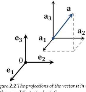
The orthonormal basis ℇ allows for the expression of any vector 𝐚 in terms of its three projected components (or coordinates) 𝑎𝑖(Figure 2.2) and can be uniquely represented by the linear combination:

10

-𝐚= 𝑎1𝐞1+𝑎2𝐞2 +𝑎3𝐞3 = � 𝑎𝑖𝐞i 3

i=1

2-8

which, employing Einstein’s summation convention (unless otherwise stated, whenever an index is repeated in the same term a summation across this index is implied) can be written as:

𝐚= 𝑎𝑖𝐞𝑖 2-9

The scalars 𝑎𝑖are termed the Cartesian (or rectangular) components of 𝐚.

This allows for the column or matrix notation of the vector 𝐚 expressed in ℇ as:

𝐚=�𝑎𝑎12

𝑎3

� 2-10

The gradient of a vector 𝐚 with respect to 𝒙 is denoted with the symbol ∇ and is defined:

∇x𝐚= ∂𝐚_∂𝒙i

𝑗 2-11

The cross (or vector or outer) product of the vectors 𝐚 and 𝐛 is defined by:

𝐚×𝐛= �𝑎𝑎12

𝑎3

�×�𝑏𝑏12

𝑏3

� =�𝑎𝑎23𝑏𝑏31 − 𝑎− 𝑎13𝑏𝑏23

𝑎1𝑏2 − 𝑎2𝑏1

� 2-12

and produces a new vector 𝐚×𝐛 which is orthogonal to both 𝐚 and 𝐛 (Figure 2.3). The magnitude of the cross product, which equals the area of the parallelogram defined by the vectors 𝐚 and 𝐛, is given by:

|𝐚×𝐛| = |𝐚||𝐛| sin𝜃 2-13 Figure 2.2 The projections of the vector 𝒂 in the

11

-The properties of the cross product can be summarised by:

𝐚×𝐛= −(𝐛×𝐚)

𝐚×𝐛= 𝟎, then 𝐚 and 𝐛 are linearly dependent (parallel)

(𝛼𝐚) ×𝐛=𝐚× (𝛼𝐛) =𝛼(𝐚×𝐛)

𝐚 ∙(𝐛×𝐜) =𝐛 ∙(𝐜×𝐚) =𝐜 ∙(𝐚×𝐛), (known as triple scalar product and equals volume of parallelepiped defined by 𝐚, 𝐛 and 𝐜)

𝐚× (𝐛+𝐜) = (𝐚×𝐛) + (𝐚×𝐜) =𝐚×𝐛+𝐚×𝐜

2-14

The so-called dyad of a vector pair e.g. 𝐚 and 𝐛 is given by their tensor product denoted by

𝐚⨂𝐛 and produces a second-order tensor (vectors are first order tensors). The dyad can be illustrated in Cartesian component notation as:

𝐚⨂𝐛= �𝑎𝑎12

𝑎3

�[𝑏1 𝑏2 𝑏3] =�

𝑎1𝑏1 𝑎1𝑏2 𝑎1𝑏3

𝑎2𝑏1 𝑎2𝑏2 𝑎2𝑏3

𝑎3𝑏1 𝑎3𝑏2 𝑎3𝑏3

� 2-15

The tensor product has the following properties:

(𝐚⨂𝐛)𝐜= 𝐚(𝐛 ∙ 𝐜)

(𝐚⨂𝐛)(𝐜+𝐝) =𝐚(𝐛 ∙ 𝐜+𝐛 ∙ 𝐝) = (𝐚⨂𝐛)𝐜+ (𝐚⨂𝐛)𝐝

(𝐚⨂𝐛)(𝛼𝐜) =𝛼(𝐚⨂𝐛)𝐜=𝛼(𝐛 ∙ 𝐜)𝐚

𝐜⨂(𝐚+𝐛) =𝐜⨂𝐚+𝐜⨂𝐛, and (𝐚+𝐛)⨂𝐜=𝐚⨂𝐜+𝐛⨂𝐜

(𝛼𝐚)⨂(𝛽𝐛) =𝛼𝛽(𝐚⨂𝐛)

2-16

Any second-order tensor may be expressed as a linear combination of dyads with respect to the orthonormal basis ℇ, e.g. for instance the second-order tensor 𝐀:

𝐀 =𝐴𝑖𝑗𝐞𝑖⨂𝐞𝑗 =�

𝐴11 𝐴12 𝐴13

𝐴21 𝐴22 𝐴13

𝐴31 𝐴32 𝐴33

� 2-17

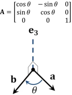
Second-order tensors are geometric objects describing linear mappings between scalars, vectors or other tensors. For instance 𝐀 may act as a rotation tensor, rotating the vector

12

-𝐚 at an angle 𝜃 around an axis coinciding with 𝐞𝟑 to the new vector 𝐛 (Figure 2.4). This type of linear mapping may be written as:

𝐀𝐚= 𝐛 2-18

where in this case the tensor 𝐀 would have the form:

𝐀=�cossin𝜃𝜃 −cossin𝜃𝜃 00

0 0 1� 2-19

The so-called (second-order) identity tensor 𝐈 can be expressed as:

𝐈=𝐞𝑖⨂𝐞𝑖 =�

1 0 0 0 1 0

0 0 1� 2-20

The inverse of a tensor 𝐀 is denoted 𝐀−1 _{and is defined such that:}

𝐀𝐀−1_=𝐀−1_{𝐀= 𝐈 2-21} The determinant of a tensor 𝐀 is denoted: det(𝐀) and has the properties:

det(𝐀𝐁) = det𝐀det𝐁, and det𝐀T _{= det𝐀}

2-22

Properties of second-order tensors can be summarised as:

𝐀+𝐁=𝐁+𝐀 𝐀+ (𝐁+𝐂) = (𝐀+𝐁) +𝐂

(−1)𝐀=−𝐀, the negative tensor

𝟎𝐚=𝒐, and 𝐀+ (−1)𝐀=𝟎, with 𝟎 the zero tensor

1𝐀=𝐈𝐀=𝟎+𝐀=𝐀 𝐀(𝐚+𝐛) =𝐀𝐚+𝐀𝐛

𝐀(𝛼𝐚) =𝛼(𝐀𝐚) = (𝛼𝐀)𝐚= 𝛼(𝐀𝐚) (𝐀+𝐁)𝐚= 𝐀𝐚+𝐁𝐚

(𝛼+𝛽)𝐀 =𝛼𝐀+𝛽𝐀

2-23

Another tensor operator is the double-dot (or double contraction) operator which yields a scalar quantity. For the two tensors 𝐀 and 𝐁 it can be written as:

13

-𝐀 ∶ 𝐁= 𝐁 ∶ 𝐀= tr(𝐀T_{𝐁) = tr(𝐁}T_{𝐀) = tr(𝐀𝐁}T_{) = tr(𝐁𝐀}T_{) 2-24} where tr(𝐀) and 𝐀T _{(with 𝐀= (𝐀}T₎T_{) denote the trace and transpose of the tensor 𝐀} respectively. Properties of the double-dot operation include:

𝐈:𝐀 = tr(𝐀)

𝐀 ∶(𝐁𝐂) = (𝐁T_{𝐀) ∶ 𝐂= (𝐀𝐂}T_{) ∶ 𝐁}

𝐀 ∶(𝐚⨂𝐛) =𝐚 ∙ 𝐀𝐛

2-25

An example use of the double dot operator is the mapping of tensor quantities along a certain direction, for instance the mapping of strain tensor 𝐄 along a texture (e.g. fibre) direction specified by the vector 𝐚 as 𝐄 ∶(𝐚⨂𝐚). In the special case when the texture vector 𝐚 is aligned with one of the directions of ℇ then the double dot operator can be thought of as a “selector” of the tensor element in that direction since 𝐄 ∶(𝐚⨂𝐚) = 𝐄 ∶

(𝐞𝑖⨂𝐞𝑖) =𝐄𝑖𝑖.

Tensors can be subjected to eigenvalue decomposition. For a second-order tensor 𝐀 the eigenvalue problem is formulated as:

𝐀𝐧𝑖 = λ𝑖𝐧𝑖, with 𝐧𝑖 ≠ 𝟎 and 𝑖= 1,2,3 (no summation) 2-26

Here the scalars λ𝑖 reflect the eigenvalues and 𝐧𝑖 the normalised eigenvectors of 𝐀. The eigenvectors 𝐧𝑖 are mutually orthogonal and thus form an orthonormal basis 𝒩 =

{𝐧1,𝐧2,𝐧3}. Since 𝒩 forms an orthonormal basis, if a tensor is symmetric the following expression, known as the spectral decomposition can be obtained:

𝐀= � λ𝑖𝐧𝑖⨂𝐧𝑖 3

𝑖=1

2-27

If 𝒩 is assumed as the orthonormal basis then (using equation 2-9) 𝐀 can be reduced to the following diagonal matrix form:

𝐀= �λ01 λ02 00

0 0 λ3

� 2-28

Since the eigenvalues λ𝑖 describe a physical property of a tensor they are independent of the chosen coordinate system. This allows for the formulation of derived invariants such as the 3 so-called principal scalar invariants, e.g. for the tensor 𝐀:

𝐼1 =λ1+λ2+λ3 = tr(𝐀)

𝐼2 =λ1λ2+λ1λ3+λ2λ3 = ₂1��tr(𝐀)�2+ tr(𝐀2)�= tr(𝐀)−1det(𝐀)

𝐼3 =λ1λ2λ3 = det(𝐀)

14

-Another tensor decomposition is the representation of a tensor 𝐀 into the sum of its so-called spherical and deviatoric part:

𝐀 =1_{3 tr}(𝐀)𝐈+ dev(𝐀) 2-30

where the deviatoric operator is defined as:

dev(𝐀) =𝐀 −1_{3 tr}(𝐀)𝐈 2-31

2.2.3

The continuum hypothesis

The main assumption underlying continuum mechanics is that the material body analysed is a continuum and is uniformly distributed throughout regions of space. In other words the material is regarded indefinitely divisible; it can be continually sub-divided into infinitesimal small elements which still exhibit the same properties as the bulk material. For a uniform material this assumption is valid up to the so-called mesoscopic scale (i.e. a scale where the dimensions of the body analysed are large in comparison to the characteristic lengths (e.g. a grain of sand, inter-atomic space) of the body 54_).

2.2.4

Motion

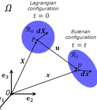
Consider a body Ωsuspended in 𝔼3 _{with orthonormal basis ℇ= {𝐞}

1,𝐞2,𝐞3} and material point 𝑃 at time 𝑡 (Figure 2.5).

15

-The body 𝛺 is in motion from its reference (Lagrangian) configuration ℛ0 at time t=0 to the new or current (Eulerian) configuration ℛ𝑡 at time t=t. The vectors 𝑿and 𝒙 are the position vectors of any point 𝑃 in 𝛺 with respect to the Lagrangian and Eulerian configuration respectively that undergo a displacement 𝐮. The motion 𝝌 of point 𝑃 is defined by an equation of the form:

𝒙= 𝝌(𝑿,𝑡) 𝑿= 𝝌−𝟏_{(𝒙,𝑡) 2-32} The displacement vector 𝐮 represents the displacement of the point 𝑃 from its original to its final position p can be defined by:

𝐮(𝑿,𝑡) =𝐱(𝑿,𝑡)− 𝑿 𝐮(𝒙,𝑡) =𝒙 − 𝑿(𝒙,𝑡) 2-33

2.2.5

Deformation

Differentiating of equation 2-32 with respect to the Lagrangian coordinates leads to:

𝜕𝒙= 𝐅𝜕𝑿 2-34

where 𝐅 represents the deformation gradient tensor as:

𝐅=_𝜕𝑿𝜕𝒙 =𝛻𝑿𝐮+𝐈 2-35

The deformation gradient tensor transforms any elementary segment 𝜕𝑿 of 𝛺 in the Lagrangian configuration into a segment ∂𝒙 in the Eulerian configuration. The inverse of

𝐅 is known as 𝐃 and is defined as:

𝐃=𝐅−1 ₌𝜕𝑿

𝜕𝒙 2-36

and transforms any elementary segment ∂𝒙 of 𝛺 in the Eulerian configuration into a segment ∂𝑿 in the Lagrangian configuration. Now consider the deformation of a volume element (Figure 2.6).

A volume element in the Lagrangian configuration d𝑉 with its sides aligned with the orthogonal basis vectors is defined by:

16

-dV = (𝜕𝑿1×𝜕𝑿2)⋅ 𝜕𝑿3 2-37

and in the Eulerian configuration:

dv = (𝜕𝒙1×𝜕𝒙2)⋅ 𝜕𝒙3 2-38

The Lagrangian and Eulerian configurations are related according to:

dv = 𝐽dV 2-39

The quantity 𝐽 is referred to as the Jacobian of the deformation gradient tensor and is defined by:

𝐽 =_{dV = det}dv �_∂𝑿�∂𝒙 = det(𝐅) 2-40

In the Lagrangian configuration no deformation has occurred and therefore 𝐽 equals 1. However 𝐽will also equal 1 during isochoric deformation (deformation without a change in volume). A material is incompressible if any deformation it undergoes is isochoric.

2.2.6

Stretch and rotation

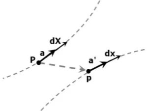
In Figure 2.7 let 𝐚 and 𝐚′ be unit vectors along d𝑿 and d𝒙 respectively and let d𝑆 be the length of an arc element in the Lagrangian configuration and d𝑠 the length of an arc segment in the Eulerian configuration.

The following relationships can then be defined:

d𝑿 = dS𝐚

d𝒙= ds𝐚′ 2-41

Equation 2-34 can then be written as ds𝐚′= 𝐅dS𝐚 leading to:

λ𝐚′ = F𝐚, with𝜆 =_d𝑆d𝑠 2-42

Where the 𝜆 is known as the stretch ratio, or simply stretch. In the special case where the vector 𝐚 is aligned with 𝐚′ the vector 𝐚 is actually an eigenvector of 𝐅and 𝜆 an eigenvalue. However the vectors 𝐚 and 𝐚′ are generally not aligned and thus the vector 𝐚 is not always the eigenvector. This means that the deformation due to 𝐅 consists of two parts: a stretch

17

-and a change in orientation. These parts can be separately expressed following what is known as polar decomposition:

𝐅 =𝐐𝐔= 𝐕𝐐 2-43

Here 𝐐 is an orthogonal tensor and 𝐔 and 𝐕 are (positive definite symmetric tensors) related to 𝐅 according to:

𝐔2 _{= 𝐅}T_𝐅

𝐕2 _=𝐅𝐅T 2-44 The tensor 𝐐 is often referred to as the rotation tensor and 𝐔 and 𝐕 are known as the right and left stretch tensors.

Now equation 2-34 can then be rewritten:

d𝒙 = (𝐐𝐔)d𝑿 =𝐐(𝐔d𝑿) 2-45

The transformation from the Lagrangian to the Eulerian configuration due to 𝐅 can thus be seen as being composed of two operations: a tri-axial stretch due to the tensor 𝐔 and a rigid body transformation (rotation, translation) due to the tensor 𝐐. Since 𝐔 is positive definite and symmetric it has one set of mutually orthogonal eigenvectors and three corresponding eigenvalues. The eigenvectors describe the direction of the eigenvalues, which are often referred to as the principal stretches 𝜆1, 𝜆2 and 𝜆3. A similar analysis can be made using the tensor 𝐕. However in this case the rigid body transformation due to 𝐐

precedes the stretch transformations due to 𝐕. The tensor 𝐕 has the same eigenvalues as

𝐔. The tensors 𝐐 (rotates, translates), 𝐔 (stretches) and 𝐕 (stretches) any elementary segment d𝑿 of 𝛺 in the Lagrangian configuration into a segment d𝒙 in the Eulerian configuration. Recall equation 2-42, squaring both sides gives:

𝜆2 _{=𝐚 ⋅(𝐅}T_{𝐅)𝐚= 𝐚 ⋅ 𝐔}2_{𝐚=𝐚 ⋅ 𝐂𝐚 2-46} The tensor 𝐔2 _{is better known as the tensor 𝐂 or the (right) Cauchy-Green tensor and can} be used to calculate 𝜆 when the vector 𝐚 is known. Similarly the inverse relationship can be obtained for the square of the tensor 𝐕2_:

1

18

-eigenvalues of the tensors 𝐁 and 𝐂 are also the same; the square of the principal stretches: 𝜆𝑖2. The invariants 𝐼𝑖 of 𝐁 and 𝐂 are defined by:

𝐼1 = tr(𝐂) =𝜆12+𝜆22+𝜆32

𝐼2 =1₂�tr(𝐂)2−tr(𝐂2)� = tr(𝐂−1) det(𝐂) =𝜆12𝜆22 +𝜆22𝜆32+𝜆12𝜆32

𝐼3 = det(𝐂) = det(𝐅T𝐅) = det(𝐅)2 = 𝐽2 = 𝜆12𝜆22𝜆32

2-48

2.2.7

Strain

The before mentioned stretch measures and the deformation gradient tensor 𝐅 are fundamental finite deformation measures defining changes of material elements during motion. However it is often convenient to derive a measure of the change in length per unit of initial length. Such a quantity is known as a strain. A large variety of strain measures have been proposed but in general their Lagrangian (left) and Eulerian (right) expressions have the form:

�𝑛1(𝐔n− 𝐈) 𝑛 ≠ 0

ln(𝐔) 𝑛 = 0 �

1

𝑛(𝐕n− 𝐈) 𝑛 ≠0

ln(𝐕) 𝑛= 0 2-49

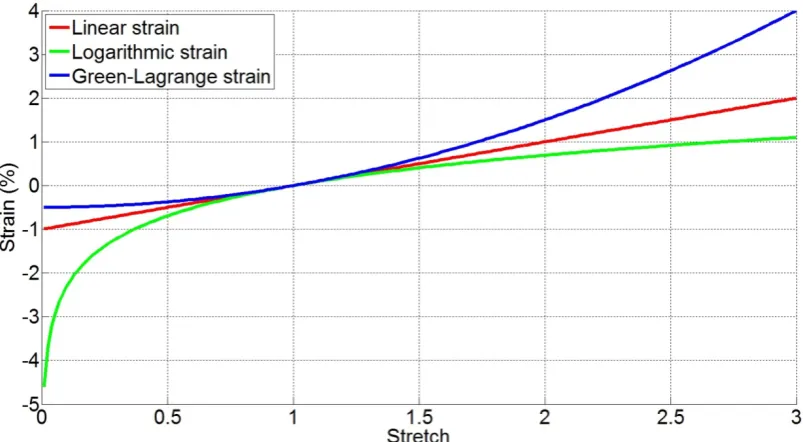
This section discusses the three most commonly used strain measures: Linear strain, Green-Lagrange strain and Logarithmic strain.

In classical engineering the linear strain tensor 𝜺 is common (also referred to as the small, infinitesimal, engineering, Cauchy or Biot strain tensor) and is defined as (𝑛 = 1 in equation 2-49):

𝛆=𝐔 − 𝐈 =1₂(𝐅T_{+𝐅)− 𝐈 2-50} For a line segment undergoing a stretch λ the linear strain is thus:𝜀 =𝜆 −1.

The Green-Lagrange strain 𝐄 is given by (𝑛= 2 in equation 2-49):

𝐄=1₂(𝐔2_{− 𝐈) =}1

2(𝐂 − 𝐈) = 1

2(𝐅T𝐅 − 𝐈) 2-51

In this case the Green-Lagrange strain in a line segment subjected to a stretch 𝜆 is:

𝐸 =1₂(𝜆2_−1).

The logarithmic (or Hencky) strain tensor 𝐇 is defined as (𝑛 = 0 in equation 2-49):

𝐇= ln(𝐔) 2-52

19

-Figure 2.8 shows the three strain measures as a function of (1D) stretch. It is clear that in the small stretch domain the three measures converge. However at larger compressive and tensile stretches the graphs diverge.

As the graph for the linear strain indicates a linear relationship with stretch exists such that for uni-axial loading interpretation of linear strain is intuitive since a stretch of 1.02 simply corresponds to a tensile strain of 2%. However linear strain is only valid for infinitesimal strain levels and is therefore not commonly used for biological soft tissue. However the Green-Lagrange strain and logarithmic strain are suitable for large finite strains and are therefore more commonly used in finite strain and biological soft tissue applications.

2.2.8

Stress

In continuum mechanics stresses in a body are due to two types of forces, external and internal forces. External forces act on part or the whole of the boundary surface. When an external force acts on the whole volume of the body (e.g. gravity) it is referred to as a body force. Internal forces act on (imaginary) surfaces within the body. Figure 2.9 shows a surface element d𝑠 belonging to the continuum body 𝛺 in the Lagrangian and an Eulerian configuration.

20

-Since stress is force over unit area, the stress due to an infinitesimal force d𝑓 acting on a surface element d𝑠 of 𝛺 can be defined as:

d𝐟= 𝐭d𝑠= 𝐓d𝑆 2-53

Then due to Newton’s law of action and reaction we obtain:

𝐭(𝒙,𝑡,𝐧) =−𝐭(𝒙,𝑡,−𝐧) 𝐓(𝑿,𝑡,𝐍) =−𝐓(𝑿,𝑡,−𝐍) 2-54

Here 𝐭 represents the Cauchy traction vector acting on the surface element d𝑠 with surface normal 𝐧 at location 𝒙. The Cauchy traction vector is the force per unit area of the current configuration. The traction vector 𝐓 is known as the first Piola-Kirchhoff traction vector and it is the force per unit area of the reference configuration.

According to Cauchy’s stress theorem there exist two unique tensors 𝛔 and 𝐏 such that:

𝐭(𝒙,𝑡,𝐧) =𝛔(𝒙,𝑡)𝐧 𝐓(𝑿,𝑡,𝐍) =𝐏(𝑿,𝑡)𝐍 2-55

The tensor 𝛔 is known as the Cauchy (or true) stress tensor and the tensor 𝐏 is referred to as the first Piola-Kirchhoff or Lagrangian stress tensor. The two tensors are related to each other as:

𝛔= 𝐽−1_𝐏𝐅T

𝐏= 𝐽𝛔𝐅−1 2-56 In matrix notation 𝛔 is:

𝛔= �𝜎𝜎1112 𝜎𝜎2122 𝜎𝜎3132

𝜎13 𝜎23 𝜎33

� 2-57

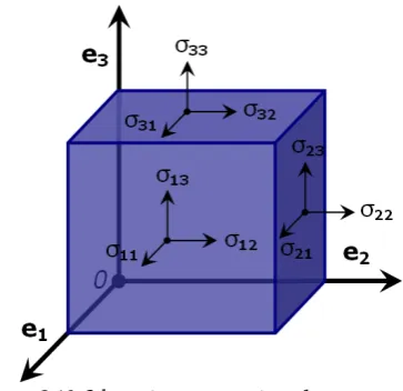
The columns of 𝛔 are the components of the traction vectors acting on planes orthogonal to the basis ℇ. Figure 2.10 shows a graphical representation of the stress components acting on an infinitesimal cubic material element of 𝛺 aligned with ℇ. Because the Cauchy

21

-stress tensor is symmetric it has six independent components (𝜎12= 𝜎21,𝜎13=

𝜎31,𝜎23= 𝜎32).

The Piola-Kirchhoff stress tensor is asymmetric and often symmetric stress formulations are preferred. However the Piola-Kirchhoff stress tensor can be decomposed as:

𝐏= 𝐅𝐒 2-58

Here the tensor 𝐒 is symmetric and is known as the second Piola-Kirchhoff stress tensor and can be related to 𝛔 and 𝐏 via:

𝐒=𝐽𝐅−1_𝛔𝐅−T_=𝐅−1_𝐏=𝐒T

𝛔= 𝐽−1_𝐅𝐒𝐅T 2-59 It is often convenient to work with the so-called Kirchoff stress tensor 𝛕 which differs from the Cauchy stress tensor by the Jacobian 𝐽:

𝛕= 𝐽𝛔 2-60

2.2.9

Strain energy

In a (thermodynamic) continuum the first law of thermodynamics states there must be a balance of both thermal and mechanical energy. Under isothermal conditions however (or when thermal effects are ignored) this reduces to balance of mechanical energy:

𝒫𝑒𝑥𝑡(𝑡) =𝑑𝒦_𝑑𝑡(𝑡)+𝑑𝛱𝑖𝑛𝑡_𝑑𝑡(𝑡) 2-61 which states that the external mechanical power 𝒫𝑒𝑥𝑡 equals the rate of change of the kinetic energy 𝒦 of the mechanical system plus the rate of change of the internal mechanical work 𝛱𝑖𝑛𝑡. The internal mechanical work 𝛱𝑖𝑛𝑡 is due to internal stresses and can be written as:

22

-𝛱𝑖𝑛𝑡(𝑡) = � Ψ𝑑𝑉 𝛺

= � Ψ𝐽−1_𝑑𝑣 𝛺

2-62

The symbol Ψ denotes a scalar function known as the Helmholtz free-energy function which, under the isothermal conditions mentioned, coincides with the internal strain energy and can therefore be considered solely a function of a deformation or strain tensor. For an isotropic material we may thus express the Helmholtz free-energy function purely in terms of deformation measures such the tensors 𝐅, 𝐂, the invariants 𝐼𝑖 or the principal stretches 𝜆𝑖:

Ψ(𝐅) =Ψ(𝐂) =Ψ(𝐼1,𝐼2,𝐼3) =Ψ(𝜆1,𝜆2,𝜆3) 2-63

Because of this the Helmholtz free-energy function is often referred to as the strain-energy density function. Strain-strain-energy density functions are important for the formulation of constitutive laws since derivatives of it with respect to deformation measures yield stress measures. For homogeneous hyperelastic materials for instance the following relations can be made between Ψ and selected stress tensors:

𝐏=∂Ψ_∂𝐅(𝐅)= 2𝐅∂Ψ_∂𝐂(𝐂)

𝐒=𝐅−1∂Ψ(𝐅)

∂𝐅 = 2

∂Ψ(𝐂)

∂𝐂 =

∂Ψ(𝐄)

∂𝐄

𝛔= 𝐽−1_{𝐅 �}∂Ψ(𝐅)

∂𝐅 �

T

= 2𝐽−1_𝐅∂Ψ(𝐂)

∂𝐂 𝐅T

𝛕= 2𝐅∂Ψ_{∂𝐂 𝐅}(𝐂) T _{= 2𝐁}∂Ψ(𝐁)

∂𝐁 =

∂Ψ(𝛆)

∂𝛆

2-64

2.2.10

Constitutive equations

2.2.10.1 Introduction

23

-deformation. The term elasticity refers to a materials ability to recover from deformation once the stresses are removed and the term plasticity refers to a materials ability to undergo irreversible deformations. The current thesis focusses on elastic soft tissue behaviour and as such plasticity is not discussed here. Instead this section discusses the following constitutive theories: linear elasticity, non-linear elasticity and viscoelasticity.

2.2.10.2 Linear elasticity

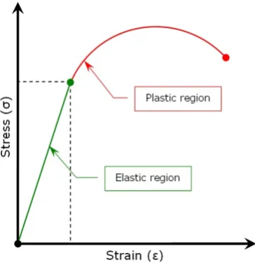
An elastic solid that undergoes an infinitesimal deformation and for which the governing material law is linear is called a linear elastic solid55_{. Figure 2.11 shows the shape of a}

typical stress strain curve for a uni-axial tensile test on such a linear elastic solid material. The theory of linear elasticity states that the stress at any time is directly proportional to the strain and is independent of strain history. Therefore for a certain deformed configuration there exists a single unique stress state. The stress (σ) strain (ε) relationship in Figure 2.11 can be described by an equation of the form σ=Eε. This constitutive equation is a special case of a material law known as Hooke’s law. The constant E is known as the Young’s Modulus and defines the slope of the curve and is effectively the stiffness of the material. The generalised form of Hooke’s law for a homogeneous and isotropic linear elastic material relates the Cauchy stress 𝛔 to the linear strain tensor 𝛆 as:

𝛔=λ𝐈tr(𝛆) +2µ𝛆

𝛆=_{2µ �𝛔 −}1 _{3λ+ 2}λ _µtr(𝛔)𝐈� 2-65

These relationships introduce two elastic moduli µ and λ referred to as the Lamé parameters. Alternatively this relationship can be written in matrix form:

24

-⎣ ⎢ ⎢ ⎢ ⎡_σσ11₂₂

σ33

σ23

σ31

σ12⎦

⎥ ⎥ ⎥ ⎤ = ⎣ ⎢ ⎢ ⎢ ⎢

⎡2µ_λ+λ λ

0 0 0

λ 2µ+λ

λ 0 0 0 λ λ 2µ+λ

0 0 0 0 0 0 µ 0 0 0 0 0 0 µ 0 0 0 0 0 0

µ⎦⎥ ⎥ ⎥ ⎥ ⎤ ⎣ ⎢ ⎢ ⎢ ⎢ ⎡ε_ε11₂₂

ε33

2ε23

2ε31

2ε12⎦

⎥ ⎥ ⎥ ⎥ ⎤ ⎣ ⎢ ⎢ ⎢ ⎢ ⎡ε_ε11₂₂

ε33

2ε23

2ε31

2ε12⎦

⎥ ⎥ ⎥ ⎥ ⎤

=_𝐸1

⎣ ⎢ ⎢ ⎢ ⎢ ⎡ _−𝜈1

−𝜈 0 0 0 −𝜈 1 −𝜈 0 0 0 −𝜈 −𝜈 1 0 0 0 0 0 0 2(1 +𝜈)

0 0 0 0 0 0 2(1 +𝜈)

0 0 0 0 0 0 2(1 +𝜈) ⎦⎥

⎥ ⎥ ⎥ ⎤ ⎣ ⎢ ⎢ ⎢ ⎡σ_σ11₂₂

σ33

σ23

σ31

σ12⎦

⎥ ⎥ ⎥ ⎤

2-66

where 𝐸 and 𝜈 represent the Young’s modulus and Poison’s ratio respectively which can be related to the Lamé parameters using:

𝐸= µ(3λ_λ++_µ2µ)

𝜈 = _2(λλ_+µ)

λ=₁2₋µ𝜈_2𝜈= _{(1 +𝜈)(1}𝐸𝜈 _−2𝜈)

µ=λ(1₂−_𝜈2𝜈) =_{2(1 +}𝐸 _𝜈)

𝜅=λ+2₃µ= _{3(3µ − 𝐸}µ𝐸 _{) =}2₃₍₁µ(𝜈₋+ 1)_2𝜈)

2-67

where 𝜅 represents the bulk modulus. The parameter µ is also known as the shear modulus.

Many engineering materials can be successfully modelled using linear elasticity especially at infinitesimal strains. However for materials like polymers, rubbers and biological soft tissues which are non-linear and capable of undergoing large deformations the infinitesimal analysis and linearity assumptions are not valid.

2.2.10.3 Non-linear elasticity

25

-A general formulation is the so-called polynomial hyperelastic60 _{given by the}

strain-energy density function:

Ψ(𝐼1,𝐼2) = � 𝑐𝑖𝑗(𝐼1−3)𝑖(𝐼2 −3)𝑗 𝑁

𝑖,𝑗=0

2-68

Here 𝐼𝑖 are the strain invariants (equation 2-48) and 𝑐𝑖𝑗 are material constants (with 𝑐00 =

0). Various strain energy formulations can be obtained by using different combinations of these constants. For instance for 𝑁= 1 and 𝑐11= 0 the formulation reduces to the so called Mooney-Rivlin hyperelastic:

Ψ(𝐼1,𝐼2) =𝑐01(𝐼1−3)+𝑐10(𝐼2 −3) 2-69

If in addition 𝑐10 = 0 the model reduces to the Neo-Hookean hyperelastic:

Ψ(𝐼1) =𝑐01(𝐼1−3) 2-70

Another commonly used model is the Ogden hyperelastic model (see also 56, 57, 61, 62_{). Its strain energy function for incompressible materials is defined by:}

Ψ(𝜆1,𝜆2,𝜆3) =�𝜇_𝛼𝑖 𝑖�𝜆1

𝛼𝑖_+𝜆

2 𝛼𝑖_+𝜆

3 𝛼𝑖_−3�

𝑁

𝑖=1

2-71

Here 𝑁 is an integer (> 0) dictating the model order and in practise often 𝑁< 4 since

𝑁= 3 is generally sufficient to achieve appropriate correlation56, 57, 61_{. The constants 𝜇}

𝑖 are the shear moduli and 𝛼𝑖 are dimensionless constants. Again various strain energy formulations can be obtained by using different combinations of constants. When the following combination of constants is used: 𝑁= 2, 𝛼1 = 2, 𝛼2 =−2, the Ogden model reduces to the Mooney-Rivlin model (equivalent to equation 2-69):

Ψ(𝜆1,𝜆2,𝜆3) =𝜇₂1(𝜆12+𝜆22+𝜆23−3)−𝜇₂2(𝜆−21 +𝜆2−2+𝜆−23 −3) 2-72

When instead 𝑁 = 1 and 𝛼1 = 2 then the Ogden model reduces to a Neo-Hookean model (equivalent to equation 2-70):

Ψ(𝜆1,𝜆2,𝜆3) =𝜇₂(𝜆12+𝜆22+𝜆23−3) 2-73

The above models are for incompressible materials (𝐽= 1). For compressible hyperelastic materials we can decompose the deformation gradient tensor 𝐅 and Cauchy strain tensor 𝐂 into a volumetric (volume changing, dilation) part, and an isochoric (volume preserving, distortional, deviatoric) part56_:

26

-𝐂= 𝐽23𝐂�

Here J1/3 _{and J}2/3 _{are associated with volumetric deformation and the so called modified}

deformation gradient tensor 𝑭� and the modified strain tensor 𝐂� are associated with the isochoric deformation (thus det�𝑭��= det�𝐂��= 1). Modified strain invariants and principal stretches may now be defined as:

𝐼�1 =𝐽−23𝐼1

𝐼�2 =𝐽−43𝐼2

𝐼�3 = 1

𝜆̃𝑖 =𝐽−13𝜆𝑖

2-75

The strain-energy functions can also be rewritten as the sum of an isochoric part Ψiso�𝐂�� and a volumetric part Ψvol(𝐽) which is a function of the Jacobian:

Ψ�𝐂�,𝐽�= Ψiso�𝐂��+Ψvol(𝐽)

Ψ(𝜆1,𝜆2,𝜆3) =Ψ�𝜆̃1,𝜆̃2,𝜆̃3,𝐽�= Ψiso�𝜆̃1,𝜆̃2,𝜆̃3�+Ψvol(𝐽)

2-76

Various forms of Ψvol(𝐽) have been proposed including the following, which is common in finite element implementations, such as FEBio (FEBio, Musculoskeletal Research Laboratories, The University of Utah, USA):

Ψvol(𝐽) =1₂𝜅(ln(𝐽)2) 2-77 where 𝜅 is the bulk modulus. Compressible hyperelastic formulations of the before mentioned constitutive laws may thus be obtained by replacing the role of 𝜆𝑖 with 𝜆̃𝑖 and by adding Ψvol(𝐽).

2.2.11

Modelling anisotropy

So far the constitutive models discussed are for isotropic materials which exhibit equivalent mechanical properties in all directions. However many biological tissues present with anisotropy. This section summarises approaches to model anisotropy with focus on hyperelastic formulations commonly implemented in finite element software.