Hierarchical Bayesian Domain Adaptation

Hierarchical Bayesian Domain Adaptation

Jenny Rose Finkel and Christopher D. Manning Computer Science Department

Stanford University Stanford, CA 94305

{jrfinkel|manning}@cs.stanford.edu

Abstract

Multi-task learning is the problem of maxi-mizing the performance of a system across a number of related tasks. When applied to mul-tiple domains for the same task, it is similar to domain adaptation, but symmetric, rather than limited to improving performance on a target domain. We present a more principled, better performing model for this problem, based on the use of a hierarchical Bayesian prior. Each domain has its own domain-specific parame-ter for each feature but, rather than a constant prior over these parameters, the model instead links them via a hierarchical Bayesian global prior. This prior encourages the features to have similar weights across domains, unless there is good evidence to the contrary. We show that the method of (Daum´e III, 2007), which was presented as a simple “prepro-cessing step,” is actually equivalent, except our representation explicitly separates hyper-parameters which were tied in his work. We demonstrate that allowing different values for these hyperparameters significantly improves performance over both a strong baseline and (Daum´e III, 2007) within both a conditional random field sequence model for named en-tity recognition and a discriminatively trained dependency parser.

1 Introduction

The goal of multi-task learning is to improve perfor-mance on a set of related tasks, when provided with (potentially varying quantities of) annotated data for each of the tasks. It is very closely related to domain adaptation, a far more common task in the natural language processing community, but with two pri-mary differences. Firstly, in domain adaptation the

different tasks are actually just different domains. Secondly, in multi-task learning the focus is on im-proving performance across all tasks, while in do-main adaptation there is a distinction between source data and target data, and the goal is to improve per-formance on the target data. In the present work we focus on domain adaptation, but like the multi-task setting, we wish to improve performance across all domains and not a single target domains. The word domain is used here somewhat loosely: it may refer to a topical domain or to distinctions that linguists might term mode (speech versus writing) or regis-ter (formal written prose versus SMS communica-tions). For example, one may have a large amount of parsed newswire, and want to use it to augment a much smaller amount of parsed e-mail, to build a higher quality parser for e-mail data. We also con-sider the extension to the task where the annotation is not the same, but is consistent, across domains (that is, some domains may be annotated with more information than others).

This problem is important because it is omni-present in real life natural language processing tasks. Annotated data is expensive to produce and limited in quantity. Typically, one may begin with a con-siderable amount of annotated newswire data, some annotated speech data, and a little annotated e-mail data. It would be most desirable if the aggregated training data could be used to improve the perfor-mance of a system on each of these domains.

From the baseline of building separate systems for each domain, the obvious first attempt at domain adaptation is to build a system from the union of the training data, and we will refer to this as a second baseline. In this paper we propose a more principled, formal model of domain adaptation, which not only outperforms previous work, but maintains attractive

performance characteristics in terms of training and testing speed. We also show that the domain adapta-tion work of (Daum´e III, 2007), which is presented as an ad-hoc “preprocessing step,” is actually equiv-alent to our formal model. However, our representa-tion of the model conceptually separates some of the hyperparameters which are not separated in (Daum´e III, 2007), and we found that setting these hyperpa-rameters with different values from one another was critical for improving performance.

We apply our model to two tasks, named entity recognition, using a linear chain conditional random field (CRF), and dependency parsing, using a dis-criminative, chart-based model. In both cases, we find that our model improves performance over both baselines and prior work.

2 Hierarchical Bayesian Domain Adaptation

2.1 Motivation

We call our model hierarchical Bayesian domain adaptation, because it makes use of a hierarchical Bayesian prior. As an example, take the case of building a logistic classifier to decide if a word is part of a person’s name. There will be a param-eter (weight) for each feature, and usually there is a zero-mean Gaussian prior over the parameter val-ues so that they don’t get too large.1 In the stan-dard, single-domain, case the log likelihood of the data and prior is calculated, and the optimal pa-rameter values are found. Now, let’s extend this model to the case of two domains, one containing American newswire and the other containing British newswire. The data distributions will be similar for the two domains, but not identical. In our model, we have separate parameters for each feature in each domain. We also have a top level parameter (also to be learned) for each feature. For each domain, the Gaussian prior over the parameter values is now centered around these top level parameters instead of around zero. A zero-mean Gaussian prior is then placed over the top level parameters. In this ex-ample, if some feature, say word=‘Nigel,’ only ap-pears in the British newswire, the corresponding weight for the American newswire will have a sim-ilar value. This happens because the evidence in the British domain will push the British parameter

1_{This can be regarded as a Bayesian prior or as weight}

reg-ularization; we adopt the former perspective here.

to have a high value, and this will in turn influence the top-level parameter to have a high value, which will then influence the American newswire to have a high value, because there will be no evidence in the American data to override the prior. Conversely, if some feature is highly indicative of isName=true for the British newswire, and of isName=false for the American newswire, then the British parameter will have a high (positive) value while the American parameter will have a low (negative) value, because in both cases the domain-specific evidence will out-weigh the effect of the prior.

2.2 Formal Model

Our domain adaptation model is based on a hierar-chical Bayesian prior, through which the domain-specific parameters are tied. The model is very general-purpose, and can be applied to any discrim-inative learning task for which one would typically put a prior with a mean over the parameters. We will build up to it by first describing a general, single-domain, discriminative learning task, and then we will show how to modify this model to construct our hierarchical Bayesian domain adaptation model. In a typical discriminative probabilistic model, the learning process consists of optimizing the log con-ditional likelihood of the data with respect to the pa-rameters,Lorig(D;θ). This likelihood function can

take on many forms: logistic regression, a condi-tional Markov model, a condicondi-tional random field, as well as others. It is common practice to put a zero-mean Gaussian prior over the parameters, leading to the following objective, for which we wish to find the optimal parameter values:

arg max

θ Lorig(D;θ)−

∑

θ2

i

2σ2 !

(1)

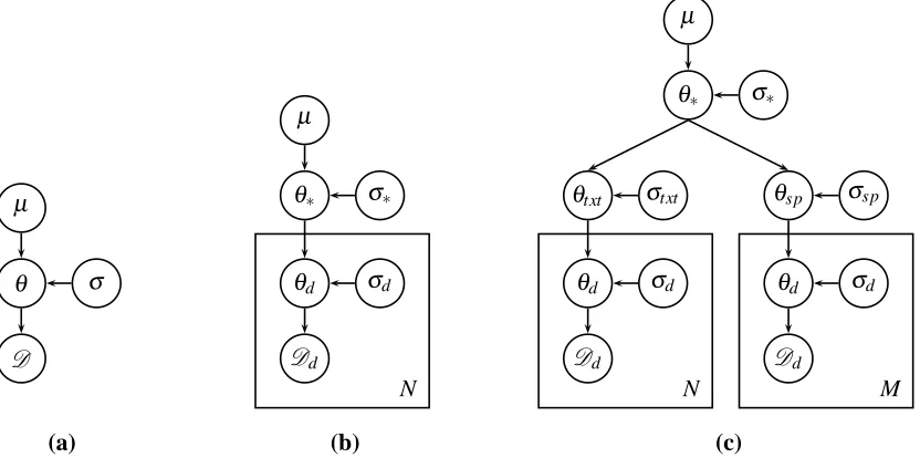
From a graphical models perspective, this looks like Figure 1(a), whereµis the mean for the prior (in our case, zero),σ2is the variance for the prior,θare the parameters, or feature weights, and D is the data. Now we will extend this single-domain model into a multi-domain model (illustrated in Figure 1(b)). Each feature weight θi is replicated once for each

domain, as well as for a top-level set of parame-ters. We will refer to the parameters for domain d as θd, with individual components θd,i, the

param-µ

θ σ

D

N

µ

θ∗ σ∗

θd σd

Dd

N M

µ

θ∗ σ∗

θtxt σtxt θsp σsp

θd σd θd σd

Dd Dd

(a) (b) (c)

Figure 1: (a) No domain adaptation. The model parameters,θ, are normally distributed, with meanµ(typically zero) and varianceσ2. The likelihood of the data,D, is dependent on the model parameters. The form of the data distribution depends on the underlying model (e.g., logistic regression, or a CRF). (b) Our hierarchical domain adaptation model. The top-level parameters,θ_∗, are normally distributed, with meanµ(typically zero) and varianceσ2

∗. There is a plate

for each domain. Within each plate, the domain-specific parameters,θ_dare normally distributed, with mean θ_∗and variance σ_d2. (c) Our hierarchical domain adaptation model, with an extra level of structure. In this example, the domains are further split into text and speech super-domains, each of which has its own set of parameters (θtxtandσtxt for text andθspandσspfor speech).θdis normally distributed with meanθtxt if domain d is in the text super-domain, andθspif it is in the speech super-domain.

eters. First, we place a zero-mean Gaussian prior over the top level parameters θ_∗. Then, these top level parameters are used as the mean for a Gaussian prior placed over each of the domain-specific param-etersθd. These domain-specific parameters are then

the parameters used in the original conditional log likelihood functions for each domain. The domain-specific parameter values jointly influence an appro-priate value for the higher-level parameters. Con-versely, the higher-level parameters will largely de-termine the domain-specific parameters when there is little or no evidence from within a domain, but can be overriden by domain-specific evidence when it clearly goes against the general picture (for instance Leeds is normally a location, but within the sports domain is usually an organization (football team)).

The beauty of this model is that the degree of in-fluence each domain exerts over the others, for each parameter, is based on the amount of evidence each domain has about that parameter. If a domain has a lot of evidence for a feature weight, then that evi-dence will outweigh the effect of the prior. However, when a domain lacks evidence for a parameter the opposite occurs, and the prior (whose value is deter-mined by evidence in the other domains) will have a

greater effect on the parameter value.

To achieve this, we modify the objective func-tion. We now sum over the log likelihood for all do-mains, including a Gaussian prior for each domain, but which is now centered around θ_∗, the top-level parameters. Outside of this summation, we have a Gaussian prior over the top-level parameters which is identical to the prior in the original model:

Lhier(D;θ) = (2)

∑

d

Lorig(Dd;θd)−

∑

(θd,i−θ∗,i)2

2σ2

d

! −

∑

i

(θ∗,i)2

2σ2 ∗ where σ_d2 and σ_∗2 are variances on the priors over the parameters for all the domains, as well as the top-level parameters. The graphical models repre-sentation is shown in Figure 1(b).

undi-rected, conditional random field-based models. The directed domain adaptation model can be viewed as a model of the parameters, and those parameter weights are used by the underlying data model. In Figure 1, the entire data model is represented by a single node,D, conditioned on the parameters,θ or θd. The form of that model can then be almost

any-thing, including an undirected model.

From an implementation perspective, the objec-tive function is not much more difficult to implement than the original single-domain model. For all of our experiments, we optimized the log likelihood using L-BFGS, which requires the function value and par-tial derivatives of each parameter. The new parpar-tial derivatives for the domain-specific parameters (but not the top-level parameters) utilize the same par-tial derivatives as in the original model. The only change in the calculations is with respect to the pri-ors. The partial derivatives for the domain-specific parameters are:

∂Lhier(D;θ)

∂θd,i

=∂Ld(Dd,θd)

∂θd,i −

θd,i−θ∗,i

σ2

d

(3)

and the derivatives for the top level parameters θ_∗ are:

∂Lhier(D;θ)

∂θ∗,i

=

∑

d

θ∗,i−θd,i

σ2

d

! −θ_σ∗₂,i

∗

(4)

This function is convex. Once the optimal param-eters have been learned, the top level paramparam-eters can be discarded, since the runtime model for each domain is the same as the original (single-domain) model, parameterized by the parameters learned for that domain in the hierarchical model. However, it may be useful to retain the top-level parameters for use in adaptation to further domains in the future.

In our model there are d extra hyper-parameters which can be tuned. These are the variancesσ_d2for each domain. When this value is large then the prior has little influence, and when set high enough will be equivalent to training each model separately. When this value is close to zero the prior has a strong in-fluence, and when it is sufficiently close to zero then it will be equivalent to completely tying the param-eters, such thatθd1,i=θd2,ifor all domains. Despite having many more parameters, for both of the tasks on which we performed experiments, we found that our model did not take much more time to train that a baseline model trained on all of the data concate-nated together.

2.3 Model Generalization

The model as presented thus far can be viewed as a two level tree, with the top-level parameters at the root, and the domain-specific ones at the leaves. However, it is straightforward to generalize the model to any tree structure. In the generalized version, the domain-specific parameters would still be at the leaves, the top-level parameters at the root, but new mid-level parameters can be added based on beliefs about how similar the various domains are. For instance, if one had four datasets, two of which contained speech data and two of which con-tained newswire, then it might be sensible to have two sets of mid-level parameters, one for the speech data and one for the newswire data, as illustrated in Figure 1(c). This would allow the speech domains to influence one another more than the newswire do-mains, and vice versa.

2.4 Formalization of (Daum´e III, 2007)

As mentioned earlier, our model is equivalent to that presented in (Daum´e III, 2007), and can be viewed as a formal version of his model.2 In his presenta-tion, the adapation is done through feature augmen-tation. Specifically, for each feature in the original version, a new version is created for each domain, as well as a general, domain-independent version of the feature. For each datum, two versions of each orig-inal feature are present: the version for that datum’s domain, and the domain independent one.

The equivalence between the two models can be shown with simple arithmetic. Recall that the log likelihood of our model is:

∑

d

Lorig(Dd;θd)−

∑

(θd,i−θ∗,i)2

2σ_d2 !

−

∑

i

(θ∗,i)2

2σ2 ∗ We now introduce a new variableψd=θd−θ∗, and plug it into the equation for log likelihood:

∑

d

Lorig(Dd;ψd+θ∗)−

∑

i

(ψd,i)2

2σ2

d

! −

∑

i

(θ∗,i)2

2σ2 ∗ The result is the model of (Daum´e III, 2007), where theψd are the domain-specific feature weights, and

θd are the domain-independent feature weights. In

his formulation, the variances σ_d2=σ_∗2 for all do-mains d.

This separation of the domain-specific and inde-pendent variances was critical to our improved per-formance. When using a Gaussian prior there are

two parameters set by the user: the mean, µ (usu-ally zero), and the variance, σ2. Technically, each of these parameters is actually a vector, with an en-try for each feature, but almost always the vectors are uniform and the same parameter is used for each feature (there are exceptions, e.g. (Lee et al., 2007)). Because Daum´e III (2007) views the adaptation as merely augmenting the feature space, each of his features has the same prior mean and variance, re-gardless of whether it is domain specific or indepen-dent. He could have set these parameters differently, but he did not.3 In our presentation of the model, we explicitly represent different variances for each domain, as well as the top level parameters. We found that specifying different values for the domain specific versus domain independent variances sig-nificantly improved performance, though we found no gains from using different values for the differ-ent domain specific variances. The values were set based on development data.

3 Named Entity Recognition

For our first set of experiments, we used a linear-chain, conditional random field (CRF) model, trained for named entity recognition (NER). The use of CRFs for sequence modeling has become stan-dard so we will omit the model details; good expla-nations can be found in a number of places (Lafferty et al., 2001; Sutton and McCallum, 2007). Our fea-tures were based on those in (Finkel et al., 2005).

3.1 Data

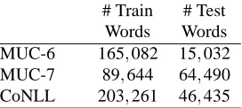
We used three named entity datasets, from the CoNLL 2003, MUC-6 and MUC-7 shared tasks. CoNLL is British newswire, while MUC-6 and MUC-7 are both American newswire. Arguably MUC-6 and MUC-7 should not count as separate domains, but because they were annotated sepa-rately, for different shared tasks, we chose to treat them as such, and feel that our experimental results justify the distinction. We used the standard train and test sets for each domain, which for CoNLL cor-responds to the (more difficult) testb set. For details about the number of training and test words in each dataset, please see Table 1.

One interesting challenge in dealing with both CoNLL and MUC data is that the label sets differ.

3_{Although he alludes to the potential for something similar}

in the last section of his paper, when discussing the kerneliza-tion interpretakerneliza-tion of his approach.

# Train # Test

Words Words

MUC-6 165,082 15,032

MUC-7 89,644 64,490

CoNLL 203,261 46,435

Table 1: Number of words in the training and test sets for each of the named entity recognition datasets.

CoNLL has four classes: person, organization, lo-cation, and misc. MUC data has seven classes: per-son, organization, location, percent, date, time, and money. They overlap in the three core classes (per-son, organization, and location), but CoNLL has one additional class and MUC has four additional classes.

The differences in the label sets led us to perform two sets of experiments for the baseline and hier-archical Bayesian models. In the first set of exper-iments, at training time, the model allows any la-bel from the union of the lala-bel sets, regardless of whether that label was legal for the domain. At test time, we would ignore guesses made by the model which were inconsistent with the allowed labels for that domain.4 In the second set of experiments, we restricted the model at training time to only allow legal labels for each domain. At test time, the do-main was specified, and the model was once again restricted so that words would never be tagged with a label outside of that domain’s label set.

3.2 Experimental Results and Discussion

In our experiments, we compared our model to sev-eral strong baselines, and the full set of results is in Table 2. The models we used were:

TARGETONLY. Trained and tested on only the data for that domain.

ALLDATA. Trained and tested on data from all do-mains, concatenated into one large dataset.

ALLDATA*. Same as ALL DATA, but restricted

possible labels for each word based on domain.

DAUME07. Trained and tested using the same tech-nique as (Daum´e III, 2007). We note that they present results using per-token label accuracy, while we used the more standard entity preci-sion, recall, and F score (as in the CoNLL 2003 shared task).

4_{We treated them identically to the background symbol. So,}

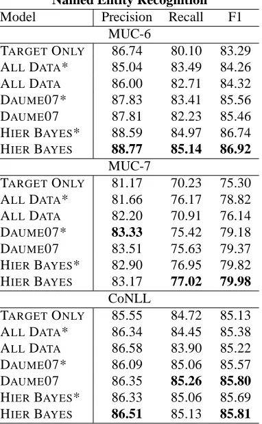
Named Entity Recognition

Model Precision Recall F1

MUC-6

TARGETONLY 86.74 80.10 83.29

ALLDATA* 85.04 83.49 84.26

ALLDATA 86.00 82.71 84.32

DAUME07* 87.83 83.41 85.56

DAUME07 87.81 82.23 85.46

HIERBAYES* 88.59 84.97 86.74

HIERBAYES 88.77 85.14 86.92

MUC-7

TARGETONLY 81.17 70.23 75.30

ALLDATA* 81.66 76.17 78.82

ALLDATA 82.20 70.91 76.14

DAUME07* 83.33 75.42 79.18

DAUME07 83.51 75.63 79.37

HIERBAYES* 82.90 76.95 79.82

HIERBAYES 83.17 77.02 79.98

CoNLL

TARGETONLY 85.55 84.72 85.13

ALLDATA* 86.34 84.45 85.38

ALLDATA 86.58 83.90 85.22

DAUME07* 86.09 85.06 85.57

DAUME07 86.35 85.26 85.80

HIERBAYES* 86.33 85.06 85.69

HIERBAYES 86.51 85.13 85.81

Table 2: Named entity recognition results for each of the models. With the exception of the TARGETONLYmodel, all three datasets were combined when training each of the models.

DAUME07*. Same as DAUME07, but restricted possible labels for each word based on domain.

HIER BAYES. Our hierarchical Bayesian domain adaptation model.

HIER BAYES*. Same as HIER BAYES, but re-stricted possible labels for each word based on the domain.

For all of the baseline models, and for the top level-parameters in the hierarchical Bayesian model, we usedσ=1. For the domain-specific parameters, we usedσd=0.1 for all domains.

The HIER BAYES model outperformed all

base-lines for both of the MUC datasets, and tied with the DAUME07 for CoNLL. The largest improvement was on MUC-6, where HIER BAYES outperformed DAUME07*, the second best model, by 1.36%. This improvement is greater than the improvement made by that model over the ALLDATA* baseline. To as-sess significance we used a document-level paired t-test (over all of the data combined), and found that

HIER BAYES significantly outperformed all of the baselines (not including HIERBAYES*) with greater than 95% confidence.

For both the HIER BAYES and DAUME07 mod-els, we found that performance was better for the variant which did not restrict possible labels based on the domain, while the ALLDATAmodel did ben-efit from the label restriction. For HIER BAYESand DAUME07, this result may be due to the structure of the models. Because both models have domain-specific features, the models likely learned that these labels were never actually allowed. However, when a feature does not occur in the data for a particular domain, then the domain-specific parameter for that feature will have positive weight due to evidence present in the other domains, which at test time can lead to assigning an illegal label to a word. This information that a word may be of some other (un-known to that domain) entity type may help prevent the model from mislabeling the word. For example, in CoNLL, nationalities, such as Iraqi and Ameri-can, are labeled as misc. If a previously unseen na-tionality is encountered in the MUC testing data, the MUC model may be tempted to label is as a location, but this evidence from the CoNLL data may prevent that, by causing it to instead be labeled misc, a label which will subsequently be ignored.

In typical domain adaptation work, showing gains is made easier by the fact that the amount of train-ing data in the target domain is comparatively small. Within the multi-task learning setting, it is more challenging to show gains over the ALLDATA base-line. Nevertheless, our results show that, so long as the amount of data in each domain is not widely dis-parate, it is possible to achieve gains on all of the domains simultaneously.

4 Dependency Parsing

4.1 Parsing Model

We built a CRF-based model, optimizing the like-lihood of the parse, conditioned on the words and parts of speech of the sentence. At the heart of our model is the Eisner dependency grammar chart-parsing algorithm (Eisner, 1996), which allows for efficient computation of inside and outside scores. The Eisner algorithm, originally designed for gen-erative parsing, decomposes the probability of a de-pendency parse into the probabilities of each attach-ment of a dependent to its parent, and the proba-bilities of each parent stopping taking dependents. These probabilities can be conditioned on the child, parent, and direction of the dependency. We used a slight modification of the algorithm which allows each probability to also be conditioned on whether there is a previous dependent. While the unmodified version of the algorithm includes stopping probabil-ities, conditioned on the parent and direction, they have no impact on which parse for a particular sen-tence is most likely, because all words must eventu-ally stop taking dependents. However, in the modi-fied version, the stopping probability is also condi-tioned on whether or not there is a previous depen-dent, so this probability does make a difference.

While the Eisner algorithm computes locally nor-malized probabilities for each attachment decision, our model computes unnormalized scores. From a graphical models perspective, our parsing model is undirected, while the original model is directed.5 The score for a particular tree decomposes the same way in our model as in the original Eisner model, but it is globally normalized instead of locally nor-malized. Using the inside and outside scores we can compute partial derivatives for the feature weights, as well as the value of the normalizing constant needed to determine the probability of a particular parse. This is done in a manner completely analo-gous to (Finkel and Manning, 2008). Partial deriva-tives and the function value are all that is needed to find the optimal feature weights using L-BFGS.6

Features are computed over each attachment and stopping decision, and can be conditioned on the

5_{The dependencies themselves are still directed in both}

cases, it is just the underlying graphical model used to compute the likelihood of a parse which changes from a directed model to an undirected model.

6_{In (Finkel and Manning, 2008) we used stochastic gradient}

descent to optimize our weights because our function evaluation was too slow to use L-BFGS. We did not encounter this problem in this setting.

parent, dependent (or none, if it is a stopping deci-sion), direction of attachment, whether there is a pre-vious dependent in that direction, and the words and parts of speech of the sentence. We used the same features as (McDonald et al., 2005), augmented with information about whether or not a dependent is the first dependent (information they did not have).

4.2 Data

For our dependency parsing experiments, we used LDC2008T04 OntoNotes Release 2.0 data (Hovy et al., 2006). This dataset is still in development, and includes data from seven different domains, la-beled for a number of tasks, including PCFG trees. The domains span both newswire and speech from multiple sources. We converted the PCFG trees into dependency trees using the Collins head rules (Collins, 2003). We also omitted the WSJ portion of the data, because it follows a different annotation scheme from the other domains.7 _{For each of the}

remaining six domains, we aimed for an 75/25 data split, but because we divided the data using the pro-vided sections, this split was fairly rough. The num-ber of training and test sentences for each domain are specified in the Table 3, along with our results.

4.3 Experimental Results and Discussion

We compared the same four domain adaptation models for dependency parsing as we did for the named entity experiments, once again setting σ = 1.0 and σd=0.1. Unlike the named entity

experi-ments however, there were no label set discrepencies between the domains, so only one version of each domain adaptation model was necessary, instead of the two versions in that section.

Our full dependency parsing results can be found in Table 3. Firstly, we found that DAUME07, which

had outperformed the ALL DATA baseline for the sequence modeling task, performed worse than the

7_{Specifically, all the other domains use the “new” Penn}

Dependency Parsing

Training Testing TARGET ALL HIER

Range # Sent Range # Sent ONLY DATA DAUME07 BAYES

ABC 0–55 1195 56–69 199 83.32% 88.97% 87.30% 88.68%

CNN 0–375 5092 376–437 1521 85.53% 87.09% 86.41% 87.26%

MNB 0–17 509 18–25 245 77.06% 86.41% 84.70% 86.71%

NBC 0–29 552 30–39 149 76.21% 85.82% 85.01% 85.32%

PRI 0–89 1707 90–112 394 87.65% 90.28% 89.52% 90.59%

VOA 0–198 1512 199–264 383 89.17% 92.11% 90.67% 92.09%

Table 3: Dependency parsing results for each of the domain adaptation models. Performance is measured as unlabeled attachment accuracy.

baseline here, indicating that the transfer of infor-mation between domains in the more structurally complicated task is inherently more difficult. Our model’s gains over the ALL DATA baseline are quite small, but we tested their significance using a sentence-level paired t-test (over all of the data com-bined) and found them to be significant at p<10−5. We are unsure why some domains improved while others did not. It is not simply a consequence of training set size, but may be due to qualities of the domains themselves.

5 Related Work

We already discussed the relation of our work to (Daum´e III, 2007) in Section 2.4. Another piece of similar work is (Chelba and Acero, 2004), who also modify their prior. Their work is limited to two do-mains, a source and a target, and their algorithm has a two stage process: First, train a classifier on the source data, and then use the learned weights from that classifier as the mean for a Gaussian prior when training a new model on just the target data.

Daum´e III and Marcu (2006) also took a Bayesian approach to domain adaptation, but structured their model in a very different way. In their model, it is assumed that each datum within a domain is either a domain-specific datum, or a general datum, and then domain-specific and general weights were learned. Whether each datum is domain-specific or general is not known, so they developed an EM based algo-rithm for determining this information while simul-taneously learning the feature weights. Their model had good performance, but came with a 10 to 15 times slowdown at training time. Our slowest de-pendency parser took four days to train, making this model close to infeasible for learning on that data.

Outside of the NLP community there has been much similar work making use of hierarchical

Bayesian priors to tie parameters across multiple, similar tasks. Evgeniou et al. (2005) present a sim-ilar model, but based on support vector machines, to predict the exam scores of students. Elidan et al. (2008) make us of an undirected Bayesian trans-fer hierarchy to jointly model the shapes of diftrans-fer- differ-ent mammals. The complete literature on related multi-task learning is too large to fully discuss here, but we direct the reader to (Baxter, 1997; Caruana, 1997; Yu et al., 2005; Xue et al., 2007). For a more general discussion of hierarchical priors, we recom-mend Chapter 5 of (Gelman et al., 2003) and Chap-ter 12 of (Gelman and Hill, 2006).

6 Conclusion and Future Work

In this paper we presented a new model for domain adaptation, based on a hierarchical Bayesian prior, which allows information to be shared between do-mains when information is sparse, while still allow-ing the data from a particular domain to override the information from other domains when there is suf-ficient evidence. We outperformed previous work on a sequence modeling task, and showed improve-ments on dependency parsing, a structurally more complex problem, where previous work failed. Our model is practically useful and does not require sig-nificantly more time to train than a baseline model using the same data (though it does require more memory, proportional to the number of domains). In the future we would like to see if the model could be adapted to improve performance on data from a new domain, potentially by using the top-level weights which should be less domain-dependent.

Acknowledgements

References

J. Baxter. 1997. A bayesian/information theoretic model of learning to learn via multiple task sampling. In

Ma-chine Learning, volume 28.

R. Caruana. 1997. Multitask learning. In Machine

Learn-ing, volume 28.

Ciprian Chelba and Alex Acero. 2004. Adaptation of a maximum entropy capitalizer: Little data can help a lot. In EMNLP 2004.

M. Collins. 2003. Head-driven statistical models for natural language parsing. Computational Linguistics, 29(4):589–637.

Hal Daum´e III and Daniel Marcu. 2006. Domain adap-tation for statistical classifiers. Journal of Artificial

Intelligence Research.

Hal Daum´e III. 2007. Frustratingly easy domain adap-tation. In Conference of the Association for

Computa-tional Linguistics (ACL), Prague, Czech Republic.

Jason Eisner. 1996. Three new probabilistic models for dependency parsing: An exploration. In

Proceed-ings of the 16th International Conference on Compu-tational Linguistics (COLING-96), Copenhagen.

Gal Elidan, Benjamin Packer, Geremy Heitz, and Daphne Koller. 2008. Convex point estimation using undi-rected bayesian transfer hierarchies. In UAI 2008. T. Evgeniou, C. Micchelli, and M. Pontil. 2005.

Learn-ing multiple tasks with kernel methods. In Journal of

Machine Learning Research.

Jenny Rose Finkel and Christopher D. Manning. 2008. Efficient, feature-based conditional random field pars-ing. In ACL/HLT-2008.

Jenny Rose Finkel, Trond Grenager, and Christopher Manning. 2005. Incorporating non-local information into information extraction systems by gibbs sampling. In ACL 2005.

Andrew Gelman and Jennifer Hill. 2006. Data Analysis

Using Regression and Multilevel/Hierarchical Models.

Cambridge University Press.

A. Gelman, J. B. Carlin, H. S. Stern, and Donald D. B. Rubin. 2003. Bayesian Data Analysis. Chapman & Hall.

Eduard Hovy, Mitchell Marcus, Martha Palmer, Lance Ramshaw, and Ralph Weischedel. 2006. Ontonotes: The 90% solution. In HLT-NAACL 2006.

John D. Lafferty, Andrew McCallum, and Fernando C. N. Pereira. 2001. Conditional random fields: Probabilis-tic models for segmenting and labeling sequence data. In ICML 2001.

Su-In Lee, Vassil Chatalbashev, David Vickrey, and Daphne Koller. 2007. Learning a meta-level prior for feature relevance from multiple related tasks. In ICML

’07: Proceedings of the 24th international conference on Machine learning.

Ryan McDonald, Koby Crammer, and Fernando Pereira. 2005. Online large-margin training of dependency parsers. In ACL 2005.

Charles Sutton and Andrew McCallum. 2007. An in-troduction to conditional random fields for relational learning. In Lise Getoor and Ben Taskar, editors,

Intro-duction to Statistical Relational Learning. MIT Press.

Ya Xue, Xuejun Liao, Lawrence Carin, and Balaji Krish-napuram. 2007. Multi-task learning for classification with dirichlet process priors. J. Mach. Learn. Res., 8. Kai Yu, Volker Tresp, and Anton Schwaighofer. 2005.

Learning gaussian processes from multiple tasks. In