Multi Source Neural Translation

Multi-Source Neural Translation

Barret Zoph and Kevin Knight Information Sciences Institute Department of Computer Science University of Southern California {zoph,knight}@isi.edu

Abstract

We build a multi-source machine translation model and train it to maximize the probabil-ity of a target English string given French and German sources. Using the neural encoder-decoder framework, we explore several com-bination methods and report up to +4.8 Bleu increases on top of a very strong attention-based neural translation model.

1 Introduction

Kay (2000) points out that if a document is trans-lated once, it is likely to be transtrans-lated again and again into other languages. This gives rise to an in-teresting idea: a human does the first translation by hand, then turns the rest over to machine translation (MT). The translation system now has two strings as input, which can reduce ambiguity via “triangu-lation” (Kay’s term). For example, the normally ambiguous English word “bank” may be more eas-ily translated into French in the presence of a sec-ond, German input string containing the word “Flus-sufer” (river bank).

Och and Ney (2001) describe such amulti-source MT system. They first train separate bilingual MT systems F→E, G→E, etc. At runtime, they sep-arately translate input strings f and g into candi-date target stringse1ande2, then select the best one of the two. A typical selection factor is the prod-uct of the system scores. Schwartz (2008) revisits such factors in the context of log-linear models and Bleu score, while Max et al. (2010) re-rankF→E

n-best lists using n-gram precision with respect to

G→E translations. Callison-Burch (2002) exploits

hypothesis selection in multi-source MT to expand available corpora, via co-training.

Others use system combination techniques to merge hypotheses at the word level, creating the ability to synthesize new translations outside those proposed by the single-source translators. These methods include confusion networks (Matusov et al., 2006; Schroeder et al., 2009), source-side string combination (Schroeder et al., 2009), and median strings (Gonz´alez-Rubio and Casacuberta, 2010).

The above work all relies on base MT systems trained on bilingual data, using traditional meth-ods. This follows early work in sentence align-ment (Gale and Church, 1993) and word alignalign-ment (Simard, 1999), which exploited trilingual text, but did not build trilingual models. Previous authors possibly considered a three-dimensional translation table t(e|f, g) to be prohibitive.

In this paper, by contrast, we train a P(e|f, g) model directly on trilingual data, and we use that model to decode an (f, g) pair simultaneously. We view this as a kind of multi-tape transduction (Elgot and Mezei, 1965; Kaplan and Kay, 1994; Deri and Knight, 2015) with two input tapes and one output tape. Our contributions are as follows:

• We train a P(e|f, g) model directly on trilin-gual data, and we use it to decode a new source string pair (f, g) into target stringe.

• We show positive Bleu improvements over strong single-source baselines.

• We show that improvements are best when the two source languages are more distant from each other.

We are able to achieve these results using

A B C <EOS> W X Y Z <EOS> Z

Y X W

Figure 1:The encoder-decoder framework for neural machine translation (NMT) (Sutskever et al., 2014). Here, a source sen-tence C B A (presented in reverse order as A B C) is translated into a target sentence W X Y Z. At each step, an evolving real-valued vector summarizes the state of the encoder (white) and decoder (gray).

the framework of neural encoder-decoder models, where multi-target MT (Dong et al., 2015) and multi-source, cross-modal mappings have been ex-plored (Luong et al., 2015a).

2 Multi-Source Neural MT

In the neural encoder-decoder framework for MT (Neco and Forcada, 1997; Casta˜no and Casacuberta, 1997; Sutskever et al., 2014; Bahdanau et al., 2014; Luong et al., 2015b), we use a recurrent neural net-work (encoder) to convert a source sentence into a dense, fixed-length vector. We then use another re-current network (decoder) to convert that vector in a target sentence.1

In this paper, we use a four-layer encoder-decoder system (Figure 1) with long short-term memory (LSTM) units (Hochreiter and Schmidhuber, 1997) trained for maximum likelihood (via a softmax layer) with back-propagation through time (Werbos, 1990). For our baseline single-source MT system we use two different models, one of which implements the local attention plus feed-input model from Lu-ong et al. (2015b).

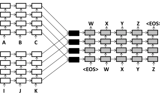
Figure 2 shows our approach to multi-source MT. Each source language has its own encoder. The question is how to combine the hidden states and cell states from each encoder, to pass on to the decoder. Blackcombinerblocks implement a function whose input is two hidden states (h1 andh2) and two cell states (c1 andc2), and whose output is a single

hid-1_{We follow previous authors in presenting the source}

sen-tence to the encoder in reverse order.

den statehand cell statec. We propose two combi-nation methods.

2.1 Basic Combination Method

The Basic method works by concatenating the two hidden states from the source encoders, applying a linear transformationWc (size 2000 x 1000), then sending its output through a tanh non-linearity. This operation is represented by the equation:

h= tanhWc[h1;h2]

(1)

Wcand all other weights in the network are learned from example string triples drawn from a trilingual training corpus.

The new cell state is simply the sum of the two cell states from the encoders.

c=c1+c2 (2)

We also attempted to concatenate cell states and ap-ply a linear transformation, but training diverges due to large cell values.

2.2 Child-Sum Method

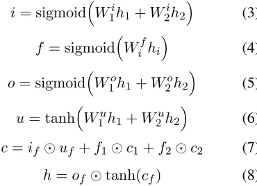
Our second combination method is inspired by the Child-Sum Tree-LSTMs of Tai et al. (2015). Here, we use an LSTM variant to combine the two hidden states and cells. The standard LSTM input, output, and new cell value are all calculated. Then cell states from each encoder get their own forget gates. The final cell state and hidden state are calculated as in a normal LSTM. More precisely:

i= sigmoidW₁ih1+W2ih2

(3)

f = sigmoidW_ifhi

(4)

o= sigmoidW₁oh1+W2oh2

(5)

u= tanhW₁uh1+W2uh2

(6)

c=if uf+f1c1+f2c2 (7) h=of tanh(cf) (8) This method employs eight new matrices (the

W’s in the above equations), each of size

A B C <EOS> W X Y Z <EOS> Z

Y X W

A B C

<EOS> W X Y Z <EOS> Z

Y X W

I J K

Figure 2:Multi-source encoder-decoder model for MT. We have two source sentences (C B A and K J I) in different languages. Each language has its own encoder; it passes its final hidden and cell state to a set ofcombiners(in black). The output of a combiner is a hidden state and cell state of the same dimension.

there are two forget gates indexed by the subscripti

that serve as the forget gates for each of the incom-ing cells for each of the encoders. In equation 5,o

represents the output gate of a normal LSTM.i,f,

o, anduare all size-1000 vectors.

2.3 Multi-Source Attention

Our single-source attention model is modeled off the local-p attention model with feed input from Luong et al. (2015b), where hidden states from the top de-coder layer can look back at the top hidden states from the encoder. The top decoder hidden state is combined with a weighted sum of the encoder hid-den states, to make a better hidhid-den state vector (h˜t), which is passed to the softmax output layer. With input-feeding, the hidden state from the attention model is sent down to the bottom decoder layer at the next time step.

The local-p attention model from Luong et al. (2015b) works as follows. First, a position to look at in the source encoder is predicted by equation 9:

pt=S·sigmoid(vTptanh(Wpht)) (9)

S is the source sentence length, andvp andWp are learned parameters, with vp being a vector of di-mension 1000, andWpbeing a matrix of dimension 1000 x 1000.

Afterptis computed, a window of size2D+ 1is looked at in the top layer of the source encoder cen-tered aroundpt(D = 10). For each hidden state in this window, we compute an alignment scoreat(s),

between 0 and 1. This alignment score is computed by equations 10, 11 and 12:

at(s) = align(ht, hs)exp

_−(s−pt)2

2σ2

(10)

align(ht, hs) = Pexp(score(ht, hs))

s0exp(score(h_t, h_s0)) (11)

score(ht, hs) =hTtWahs (12) In equation 10, σ is set to be D/2 ands is the source index for that hidden state.Wais a learnable parameter of dimension 1000 x 1000.

Once all of the alignments are calculated,ctis cre-ated by taking a weighted sum of all source hidden states multiplied by their alignment weight.

The final hidden state sent to the softmax layer is given by:

˜

ht=tanh

Wc[ht;ct]

(13) We modify this attention model to look at both source encoders simultaneously. We create a context vector from each source encoder named c1

t and c2t instead of the just ct in the single-source attention model:

˜

ht=tanh

Wc[ht;c1t;c2t]

French English German

Word tokens 66.2m 59.4m 57.0m

Word types 424,832 381,062 865,806

Segment pairs 2,378,112

Ave. segment 27.8 25.0 24.0

length (tokens)

Figure 3:Trilingual corpus statistics.

also have two separate sets of alignments and there-fore now have twoctvalues denoted byc1t andc2t as mentioned above. We also have distinctWa,vp, and

Wp parameters for each encoder.

3 Experiments

We use English, French, and German data from a subset of the WMT 2014 dataset (Bojar et al., 2014). Figure 3 shows statistics for our training set. For de-velopment, we use the 3000 sentences supplied by WMT. For testing, we use a 1503-line trilingual sub-set of the WMT test sub-set.

For the single-source models, we follow the train-ing procedure used in Luong et al. (2015b), but with 15 epochs and halving the learning rate every full epoch after the 10th epoch. We also re-scale the normalized gradient when norm>5. For training, we use a minibatch size of 128, a hidden state size of 1000, and dropout as in Zaremba et al. (2014). The dropout rate is 0.2, the initial parameter range is[-0.1, +0.1], and the learning rate is 1.0. For the normal and multi-source attention models, we ad-just these parameters to 0.3,[-0.08, +0.08], and 0.7, respectively, to adjust for overfitting.

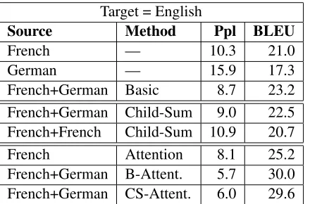
Figure 4 shows our results for target English, with source languages French and German. We see that the Basic combination method yields a +4.8 Bleu improvement over the strongest single-source, attention-based system. It also improves Bleu by +2.2 over the non-attention baseline. The Child-Sum method gives improvements of +4.4 and +1.4. We confirm that two copies of the same French input yields no BLEU improvement. Figure 5 shows the action of the multi-attention model during decoding. When our source languages are English and French (Figure 6), we observe smaller BLEU gains (up to +1.1). This is evidence that the more distinct the source languages, the better they disambiguate each other.

Target = English

Source Method Ppl BLEU

French — 10.3 21.0

German — 15.9 17.3

French+German Basic 8.7 23.2

French+German Child-Sum 9.0 22.5

French+French Child-Sum 10.9 20.7

French Attention 8.1 25.2

French+German B-Attent. 5.7 30.0

French+German CS-Attent. 6.0 29.6

Figure 4:Multi-source MT for target English, with source lan-guages French and German. Ppl reports test-set perplexity as the system predicts English tokens. BLEU is scored using the multi-bleu.perl script from Moses. For our evaluation we use a single reference and they are case sensitive.

Source 1: UNK Aspekte sind ebenfalls wichtig .

Target: UNK aspects are important , too .

Source 2: Les aspects UNK sont également importants . Figure 5: Action of the multi-attention model as the neural decoder generates target English from French/German sources (test set). Lines show strengths ofat(s).

4 Conclusion

We describe a multi-source neural MT system that gets up to +4.8 Bleu gains over a very strong attention-based, single-source baseline. We ob-tain this result through a novel encoder-vector com-bination method and a novel multi-attention sys-tem. We release the code for these experiments at www.github.com/isi-nlp/Zoph RNN.

Target = German

Source Method Ppl BLEU

French — 12.3 10.6

English — 9.6 13.4

French+English Basic 9.1 14.5

French+English Child-Sum 9.5 14.4

English Attention 7.3 17.6

French+English B-Attent. 6.9 18.6

French+English CS-Attent. 7.1 18.2

5 Acknowledgments

This work was carried out with funding from DARPA (HR0011-15-C-0115) and ARL/ARO (W911NF-10-1-0533).

References

D. Bahdanau, K. Cho, and Y. Bengio. 2014. Neural ma-chine translation by jointly learning to align and trans-late. InProc. ICLR.

O. Bojar, C. Buck, C. Federmann, B. Haddow, P. Koehn, C. Monz, M. Post, and L. Specia, editors. 2014. Proc. of the Ninth Workshop on Statistical Machine Transla-tion. Association for Computational Linguistics. C. Callison-Burch. 2002. Co-training for statistical

ma-chine translation. Master’s thesis, School of Informat-ics, University of Edinburgh.

M. A. Casta˜no and F. Casacuberta. 1997. A con-nectionist approach to machine translation. In EU-ROSPEECH.

A. Deri and K. Knight. 2015. How to make a Frenemy: Multitape FSTs for portmanteau generation. InProc. NAACL.

D. Dong, H. Wu, W. he, D. Yu, and H. Wang. 2015. Multi-task learning for multiple language translation. InProc. ACL.

C. Elgot and J. Mezei. 1965. On relations defined by generalized finite automata. IBM Journal of Research and Development, 9(1):47–68.

W. A Gale and K. W Church. 1993. A program for align-ing sentences in bilalign-ingual corpora. Computational lin-guistics, 19(1):75–102.

J. Gonz´alez-Rubio and F. Casacuberta. 2010. On the use of median string for multi-source translation. InProc. ICPR.

S. Hochreiter and J. Schmidhuber. 1997. Long short-term memory.Neural Computation, 9(8).

R. Kaplan and M. Kay. 1994. Regular models of phonological rule systems. Computational Linguis-tics, 20(3):331–378.

M. Kay. 2000. Triangulation in translation. Keynote at MT 2000 Conference, University of Exeter.

M. Luong, Q. V. Le, I. Sutskever, O. Vinyals, and L. Kaiser. 2015a. Multi-task sequence to sequence learning. InarXiv. http://arxiv.org/abs/1511.06114. M. Luong, H. Pham, and C. Manning. 2015b. Effective

approaches to attention-based neural machine transla-tion. InProc. EMNLP.

E. Matusov, N. Ueffing, and H. Ney. 2006. Computing consensus translation from multiple machine transla-tion systems using enhanced hypotheses alignment. In

Proc. EACL.

A. Max, J. Crego, and F. Yvon. 2010. Contrastive lexical evaluation of machine translation. InProc. LREC. R. Neco and M. Forcada. 1997. Asynchronous

transla-tions with recurrent neural nets. InInternational Conf. on Neural Networks, volume 4, pages 2535–2540. F. J. Och and H. Ney. 2001. Statistical multi-source

translation. InProc. MT Summit.

J. Schroeder, T. Cohn, and P. Koehn. 2009. Word lattices for multi-source translation. InProc. EACL.

L. Schwartz. 2008. Multi-source translation methods.

Proc. AMTA.

M. Simard. 1999. Text-translation alignment: Three lan-guages are better than two. InProc. EMNLP/VLC. I. Sutskever, O. Vinyals, and Q. V. Le. 2014. Sequence

to sequence learning with neural networks. In Proc. NIPS.

K. S. Tai, R. Socher, and C. Manning. 2015. Im-proved semantic representations from tree-structured long short-term memory networks. InProc. ACL. P. J. Werbos. 1990. Backpropagation through time: what

it does and how to do it. Proc. IEEE, 78(10):1550– 1560.